How to Reference Pivot Table Data in Excel (with Easy Steps)

Step 1- Creating a Pivot Table

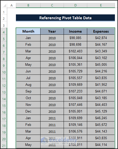
We’ll use a sample dataset in cells B4:E40.

Select the range of cells B4 to E40.

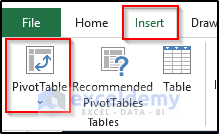
Go to the Insert tab in the ribbon.
Select PivotTable from the Tables group.

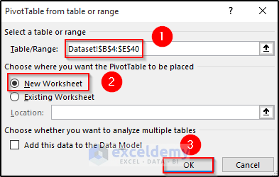
The PivotTable from table or range dialog box will appear.
Check that the range of cells is correct.
Choose where you want to place your Pivot Table.
Click on OK.

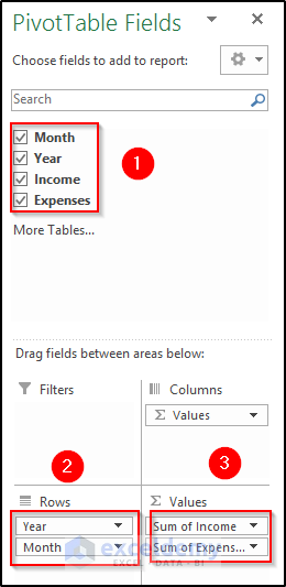
You will see a PivotTable Fields dialog box will appear.
Check all the options.
Drag the Month and Year in the Rows section and Income and Expense in the Values section.

Here’s the table.

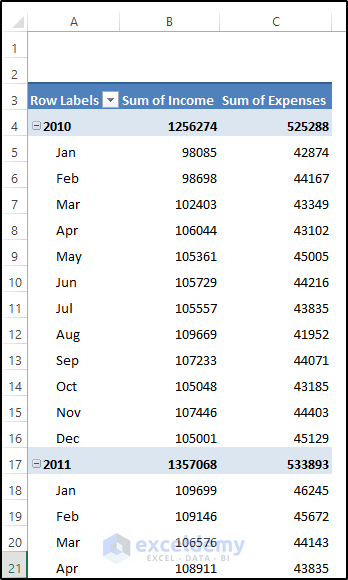
Step 2 – Calculate the Ratio of Expenses and Income for Three Different Years

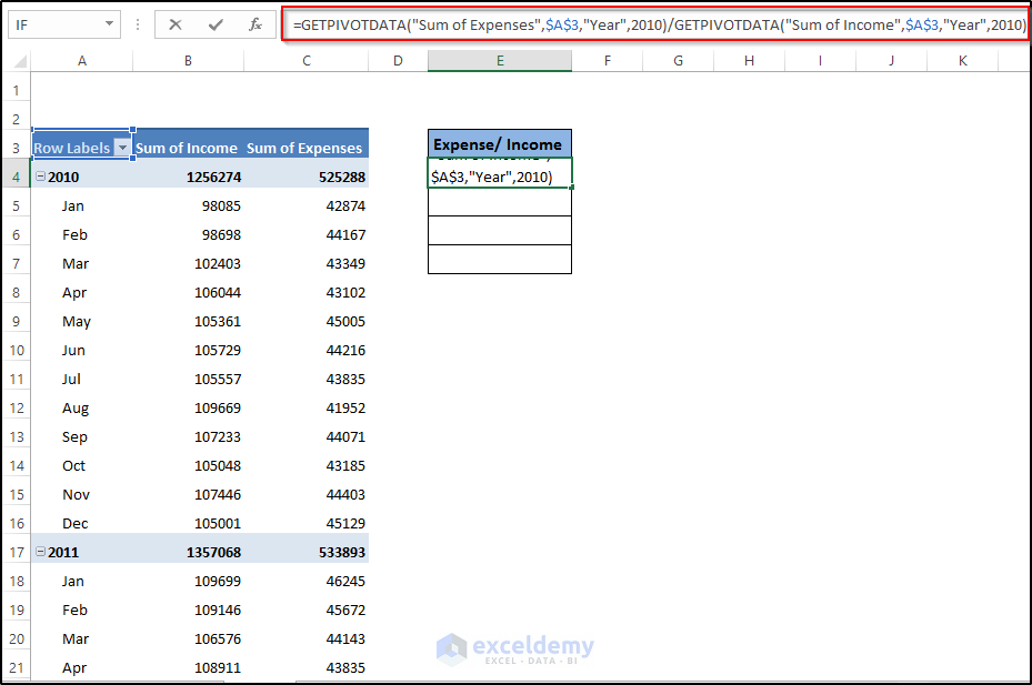
Select cell E4.
Use the following formula.

=GETPIVOTDATA("Sum of Expenses",$A$3,"Year",2010)/GETPIVOTDATA("Sum of Income",$A$3,"Year",2010)

Alternatively:

Select cell E4.
Insert the equal(=) sign.
Click on the sum of expenses for 2010 in the pivot table.
Insert the divide (/) sign.
Click on the sum of income for 2010 in the pivot table.

Press Enter to apply the formula.

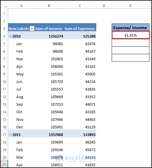
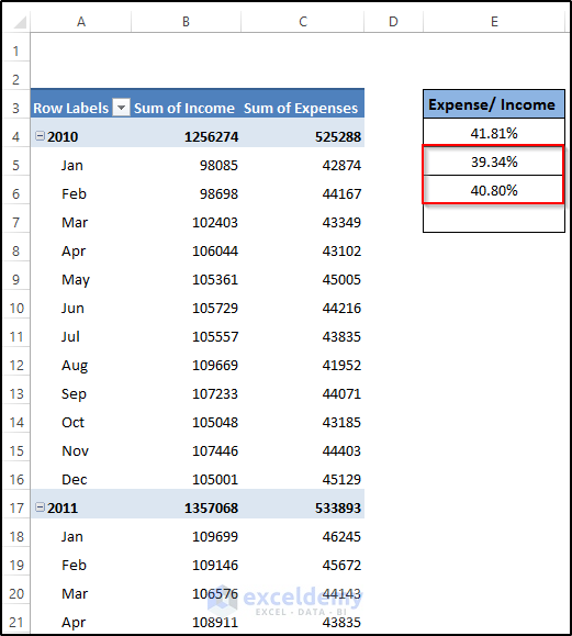
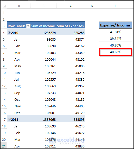
Repeat to get the ratio of expenses and income for the years 2011 and 2012 in E5 and E6, respectively.
You will get the following result.

Step 3 – Calculate the Overall Ratio of Expenses and Income

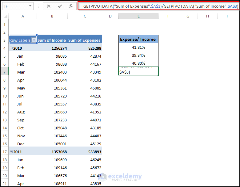
Select cell E7.
Use the following formula.

=GETPIVOTDATA("Sum of Expenses",$A$3)/GETPIVOTDATA("Sum of Income",$A$3)

Alternatively:

Select cell E7.
Insert the equal (=) sign.
Click on the grand total of the sum of expenses in the pivot table.
Insert the divide (/) sign.
Click on the grand total of the sum of income in the pivot table.

Press Enter to apply the formula.

Caution: Using the GETPIVOTDATA function has one limitation: The data that it retrieves must be visible. If you modify the pivot table so that the value used by GETPIVOTDATA is no longer visible, the formula will return an error.

How to Stop Auto-Using the GETPIVOTDATA Function

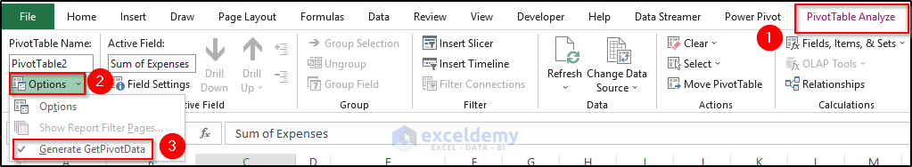
Method 1 – Using PivotTable Analyze

Steps

Select any cell in the pivot table.
Go to the PivotTable analyze tab on the ribbon.
Select the Options drop-down from the Pivot Table group.
Uncheck the Generate GetPivotData option.

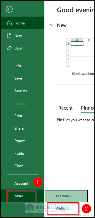
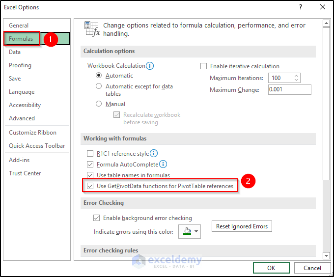
Method 2 – Utilizing Excel Options

Steps

Go to the File tab on the ribbon.
Select Options. Select More if you don’t see Options on the list.

This open up the Excel Options dialog box.
Select the Formulas option.
Uncheck Use GetPivotData functions for PivotTable references from the Working with formulas section.
Click on OK.

Things to Remember

Even if you change the layout of the pivot table, the GETPIVOTDATA function shows the correct result. For a cell reference, however, it returns an error if you modify the layout.
Excel produces the GETPIVOTDATA function whenever you click on the pivot table while editing formulas.

Download the Practice Workbook

Pivot Table Reference.xlsx

<<Go Back to Excel GETPIVOTDATA | Pivot Table in Excel | Learn Excel

Get FREE Advanced Excel Exercises with Solutions!

4 Comments

Murtaza Aug 4, 2016 at 8:32 PM

I have referenced few cells of the pivot table in another file. Whenever I open that other file containing reference, I see “#REF#” in the cells where I have references to the pivot table. As soon as I’ll open the file containing the pivot table, those cells would automatically populate the correct data. How can I fix this problem, so that I don’t have to open multiple files to see the data in my report?
- Reply
  Saquib Sep 4, 2022 at 11:37 AM
  
  Hi Murtaza,
  Your question is greatly appreciated. By following the article “How to Update Links Without Opening File in Excel”, you can easily fix your report so that you don’t have to open multiple files.
Lise Genoble Nov 18, 2021 at 9:11 PM

How do I reference a cell on another tab in the main pivot cell? When using =. . . I get the following error: ‘Cannot enter a formula for an item or field name in a PivotTable report’
- Reply
  Saquib Sep 4, 2022 at 11:58 AM
  
  Hi GENOBLE,
  Your question is greatly appreciated. You can easily fix your error by enabling Excel’s GetPivot Data function. If you want to enable Excel to use the GETPIVOTDATA function when you point to pivot table cells at the time of creating a formula, choose PivotTable Tools ➪ Analyze ➪ PivotTable ➪ Options ➪ Generate GetPivot Data command. Now, you can easily reference a cell on another tab in the main pivot cell.