Turn Messy Data Into Insights: Data Cleaning in Power BI Step-by-Step

 

Data rarely comes in perfect condition. Whether you’re importing from Excel files, databases, or web sources, you’ll likely encounter inconsistencies, missing values, and formatting issues that can derail your analysis. If not cleaned properly, these issues can lead to misleading insights. Fortunately, Power BI’s Power Query Editor makes data cleaning straightforward and repeatable.

In this tutorial, we will show you how to clean data in Power BI step by step, turning messy data into reliable insights.

1. Import Your Data in Power BI:

• Open Power BI Desktop.
• Go to the Home tab >> select Get Data.

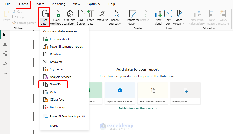
• Browse and choose your source (Excel, CSV, SQL, Web, etc.).
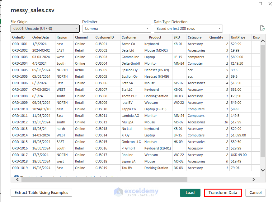
• Click Transform Data to load the dataset into the Power Query Editor.

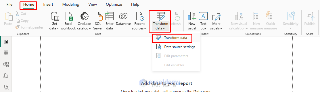
From Existing Queries:

• Go to the Home tab >> select Transform Data.
• Or right-click a table in the Fields pane >> select Edit Query.

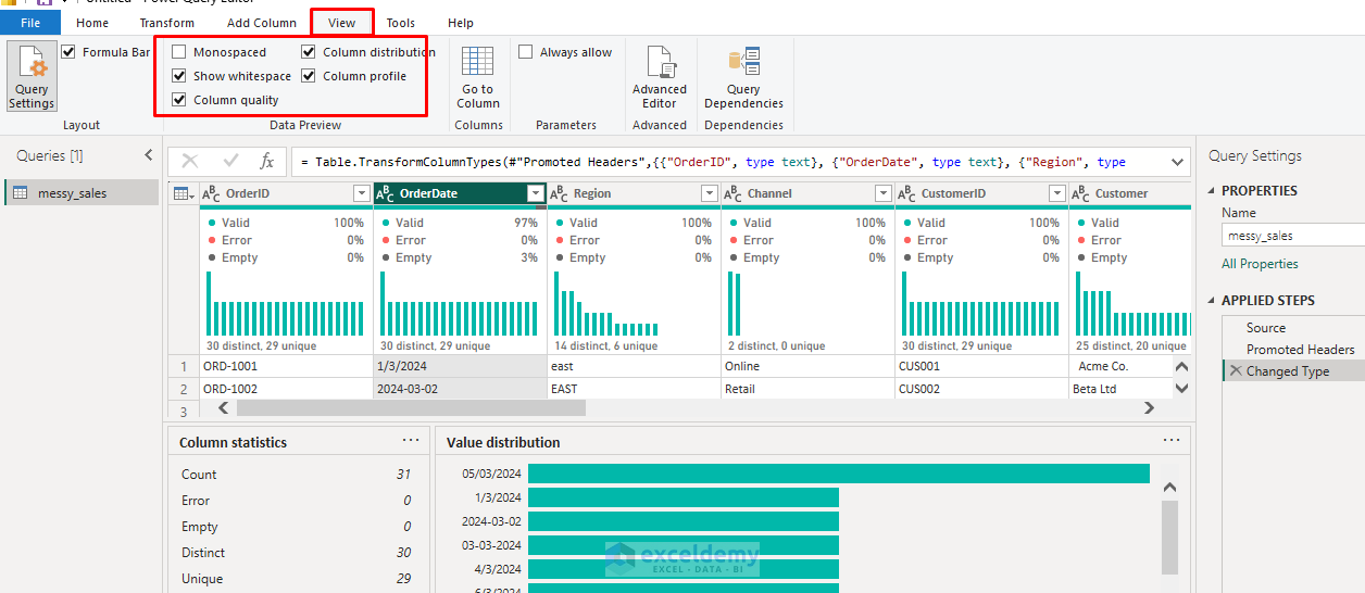
2. Turn on Data Profiling

In Power Query, you can turn on data profiling tools first to check for all types of issues.

• Go to the View tab >> select Column quality, Column distribution, and Column profile (enable for the entire dataset).
• These panels instantly reveal blanks, errors, unique values, min/max, etc., so you can target problems.

3. Promoting Headers

When importing from different sources, column names may appear as the first row of data. Also, some Excel files may have headers that start in row 2 or later. In these cases, you can promote the first row to become the headers.

• Select the table containing the headers in the first row.
• Go to the Home tab >> select Use First Row as Headers.
• Or go to the Transform tab >> select Use First Row as Headers.

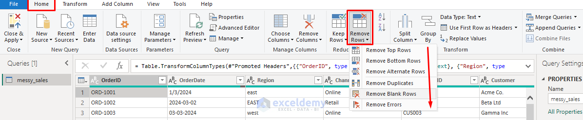
4. Remove Rows (Duplicates, Blanks, Errors, and Custom)

Remove any empty, blank, error, and duplicate rows that can inflate totals and produce misleading insights.

Remove Empty Rows:

• Go to the Home tab >> select Remove Rows >> select Remove Empty Rows.

Custom Row Removal:

• Remove Top Rows: Specify the number of rows to remove from the beginning.
• Remove Bottom Rows: Remove rows from the end.
• Remove Alternate Rows: Remove every nth row.

Remove Duplicate Rows:

• Select all relevant columns.
• Go to the Home tab >> select Remove Rows >> select Remove Duplicates.

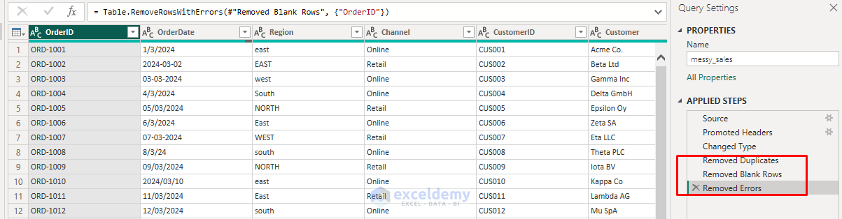
Remove Errors:

• Go to the Home tab >> select Remove Errors (or Keep Errors to investigate).

Applied Steps:

Keep Only Duplicates:

• Use the same process, but select Keep Duplicates to identify duplicate records for review.

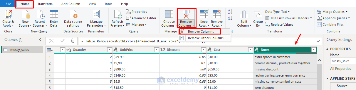
5. Remove Unnecessary Columns

Look for columns that don’t add value to your analysis and remove them.

Remove Unnecessary Columns:

• Select the columns.
• Go to the Home tab >> select Remove Columns.

6. Handle Missing Values

Messy data often has blanks or nulls. You can either replace these values, fill them down, or remove the nulls entirely.

Replace Values:

• Select the column(s) with unwanted data.
• Go to the Transform tab >> select Replace Values.
• Replace characters like $, €, USD, and € suffixes, and spaces with nothing.
• Use multiple replacements as needed.

Fill Down/Up:

• Select a column.
• Go to the Transform tab >> select Fill >> select Down or Up.

Remove Nulls:

• Click the dropdown arrow in the column header.
• Uncheck (null) or (blank).
• Click OK.

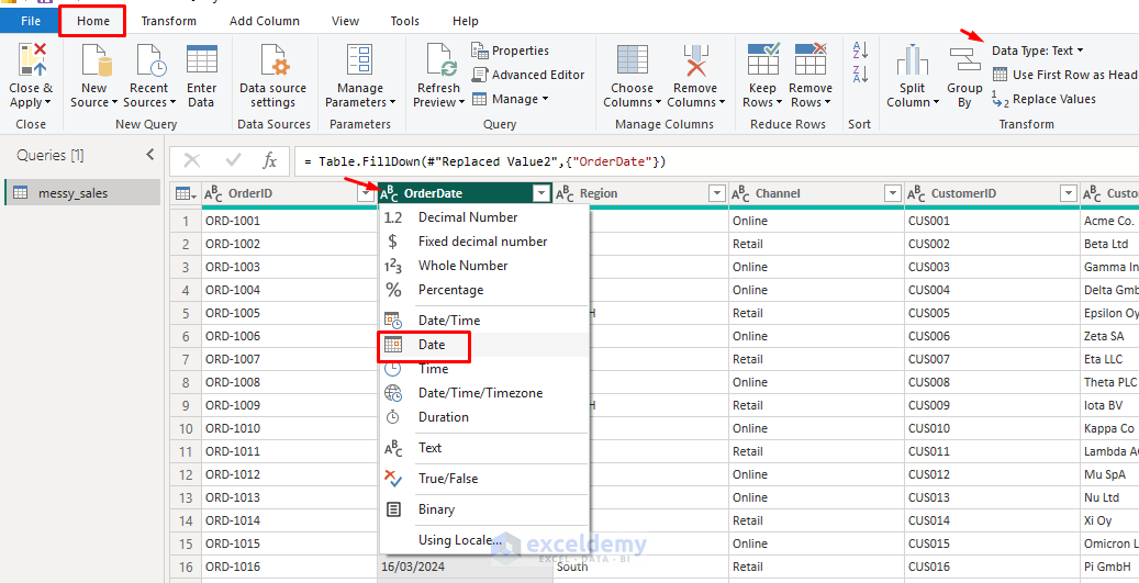
7. Standardize Formatting

Data can be inconsistent: dates might be stored as text, numbers as text, product names with mixed casing, or entries with extra spaces. Ensure your ‘Date’ column is a Date type, ‘Units’ is a Whole Number, and ‘Price’ is a Decimal.

Change Data Type:

• Icons in the column headers show the data type.
• Go to the Home tab >> select Data Type.
• Or, hover over the icon >> select the relevant Data Type.
• Select Text, Decimal Number, Date, or Whole Number based on the data types.

Use Locale:

• Hover over the icon >> select Using Locale.

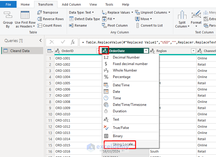
• Select the Data Type.
• Select the Country Name.

You can easily use different countries’ currencies, date formats, decimal points, etc.

Format Text:

• Select the Region, Channel, and Category columns.
• Go to the Transform tab >> select Format >> choose from:
  • Lowercase
  • Uppercase
  • Capitalize Each Word
  • Capitalize First Letter

Trim/Clean:

• Remove leading/trailing spaces or hidden characters.
• Go to the Transform tab >> select Format >> select Clean (removes non-printable characters).
• Go to the Transform tab >> select Format >> select Trim (removes extra spaces).

8. Splitting and Merging Columns

Messy datasets may combine multiple pieces of information in one column.

Split Columns:

• Select the column to split.
• Go to the Home tab >> select Split Column >> choose a method:
  • By Delimiter (comma, space, custom character)
  • By Number of Characters
  • By Positions
  • By Lowercase to Uppercase
  • By Digit to Non-Digit

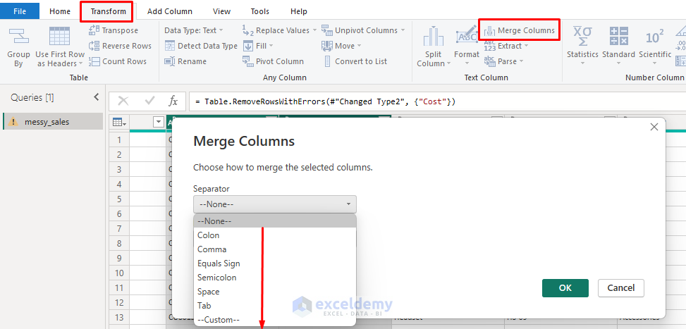
Merge Columns:

• Select multiple columns (Ctrl+click).
• Go to the Transform tab >> select Merge Columns.
• Choose a separator (space, comma, tab, or custom).

9. Create New Calculated Columns

Sometimes the raw data doesn’t contain the exact metrics you need for your analysis. You can create new columns:

• Go to the Add Column tab >> select Custom Column for formulas.
• Insert the following formula.

Revenue = [Quantity] * [UnitPrice] * (1 - [Discount])

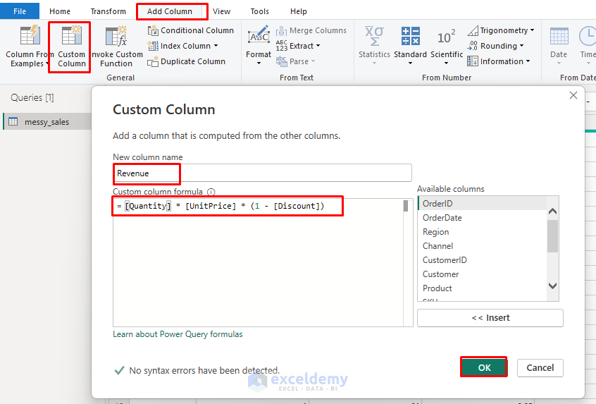
This ensures consistency instead of relying on pre-calculated values.

10. Apply Consistent Naming

Rename columns to meaningful names, such as from Cust_ID → Customer ID or Rev → Revenue ($).

• Select the column.
• Type the new column name.
• Or go to the Transform tab >> select Rename.

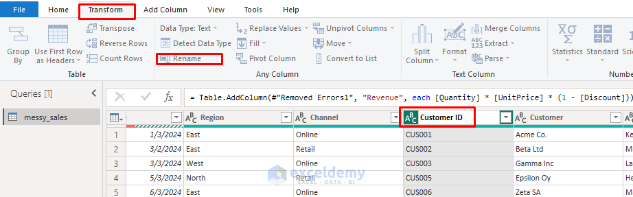
This makes reports easier for others to understand.

11. Pivot & Unpivoting Data

Convert Wide Format to Long Format (Unpivot): Use when column headers are data values (e.g., Jan–Dec, Product A–D). Converting to a tidy long table enables proper modeling, relationships, and time-intelligence/DAX measures.

• Select the columns you want to keep as identifiers.
• Go to the Transform tab >> select Unpivot Other Columns.
• This converts cross-tab data to a normalized format.

Convert Long Format to Wide Format (Pivot): Use when you want a cross-tab summary that compares categories side-by-side. This turns a field (e.g., Month or Region) into columns to aggregate and visually compare values quickly.

• Select the column containing values that will become headers.
• Go to the Transform tab >> select Pivot Column.
• Choose a value column and an aggregation method.

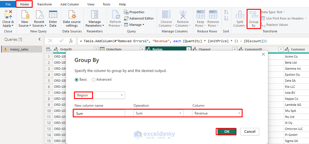
12. Group and Summarize Data

For quick insights, group rows by a column and aggregate:

• Go to the Home tab >> select Group By.
• Choose aggregations like Sum, Average, and Count.
• This helps when you have duplicates but want to preserve aggregated information.

13. Load Cleaned Data to Power BI

Once you are done with data cleaning, you can load the cleaned data into Power BI.

• Go to the Home tab >> click Close & Apply.
• Your clean dataset is now ready for building dashboards and insights.

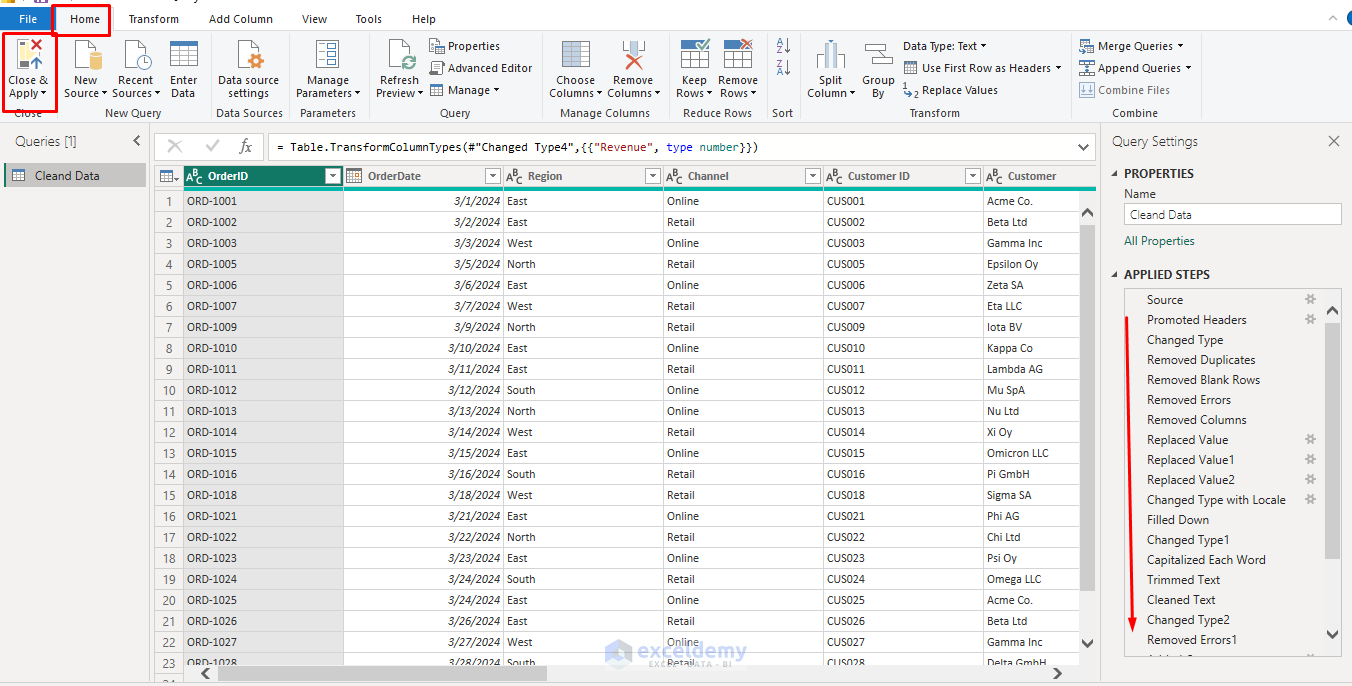
The best part about Power Query is that it saves all the applied steps, so you can change or update any step at any time.

Wrapping Up

Data cleaning may seem tedious, but it’s the foundation of reliable analysis and reporting. By using Power Query in Power BI, you can clean and structure your data efficiently. Effective data cleaning in Power BI transforms unreliable source data into trustworthy insights. With the techniques and principles shown, you’ll be equipped to handle even the messiest datasets and transform them into the foundation for compelling, accurate analysis. Power Query Editor’s step-by-step approach means you can always refine your process and adapt to new data challenges as they arise.