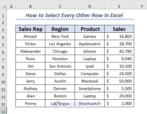
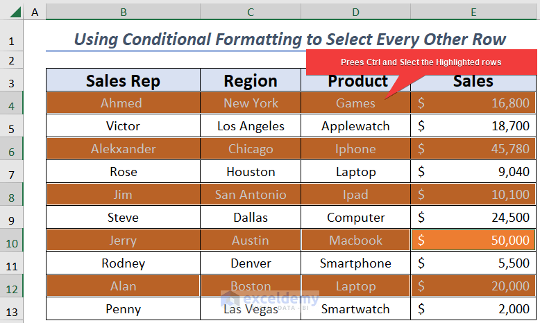
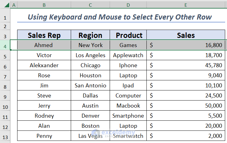
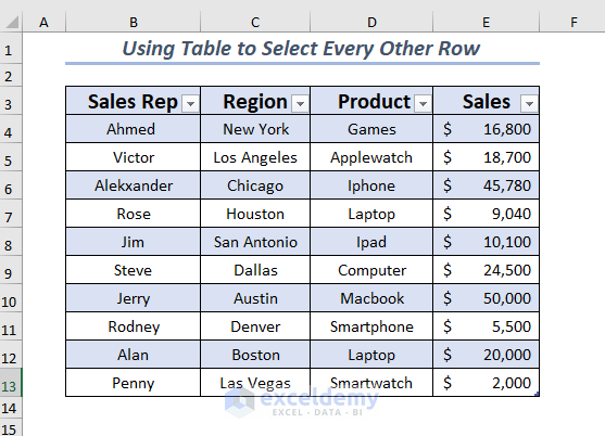
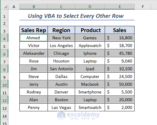
The following dataset is about the sales information of a certain tech shop. It has four columns: Sales Rep, Region, Product, and Sales. These columns show the total sales information for a particular product by a sales representative.
Method 1 – Using Conditional Formatting to Mark Selectable Cells
Steps:
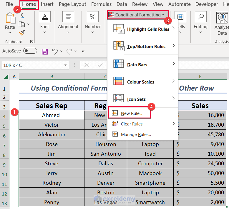
- Choose the B4:E13 cell range.
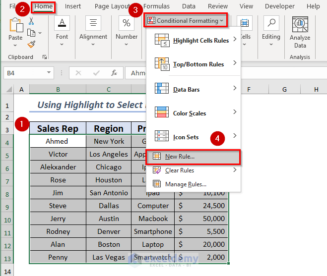
- Open the Home tab >> Go to Conditional Formatting >> select New Rule.
- A dialog box will pop up.
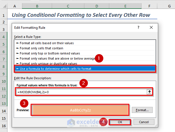
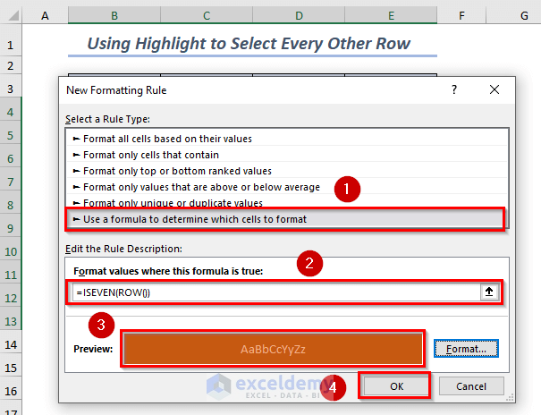
- Select Use a formula to determine which cells to format.
- Write down the following formula in the Format values where this formula is true box,
Type the formula
=MOD(ROW(B4),2)=0- Select the format of your choice.
- Click OK.
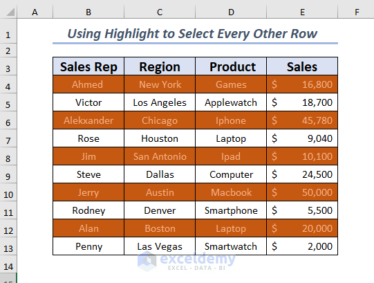
- The MOD(ROW(),2)=0 functions will Highlight every 2nd row starting from the first.
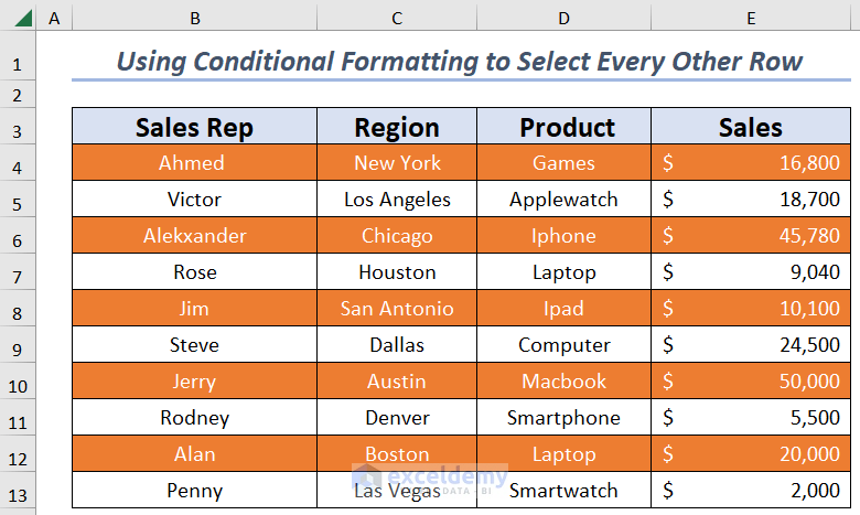
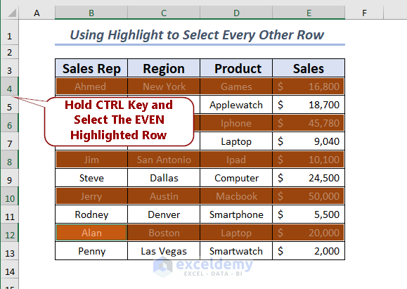
- Select the first Highlighted row then hold the CTRL key and select the rest of Highlighted rows.
Method 2 – Using Highlight Feature
Steps:
- Select the cell range that you want to Highlight and want to select.
- Open the Home tab >> Go to Conditional Formatting >> select New Rule
- A dialog box will be on the screen.
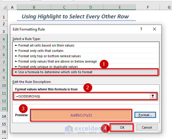
- Select Use a formula to determine which cells to format.
- Use the ISODD function. It will only Highlight the rows where the row number is odd.
Type the formula=ISODD(ROW())
- You can select the Format of your choice.
- Click OK.
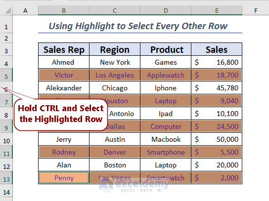
- It will Highlight the ODD number of rows.

- Select every other odd row you can select the first Highlighted row then hold the CTRL key and select the rest of Highlighted rows.
II. For EVEN Rows
Steps:
- To Highlight the even number of rows, select every other even row. Select the cell range that you want to Highlight and select later.
- Choose the B4:E13 cell range.
- Open the Home tab >> Go to Conditional Formatting >> select New Rule.
- After selecting New Rule, a dialog box will pop up.
- Choose Use a formula to determine which cells to format.
- Use the ISEVEN and the ROW function. It will only Highlight the rows where the row number is even.
Write the formula=ISEVEN(ROW())
- Choose the Format of your choice.
- Click OK.
 The EVEN rows will be Highlighted.
- To select every other even row, select the first Highlighted row then hold the CTRL key and select the rest of Highlighted rows.
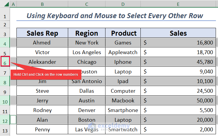
Method 3 – Using Keyboard and Mouse Shortcut
Steps:
- Select the row number, then double-click on the row number on the right side of the mouse.
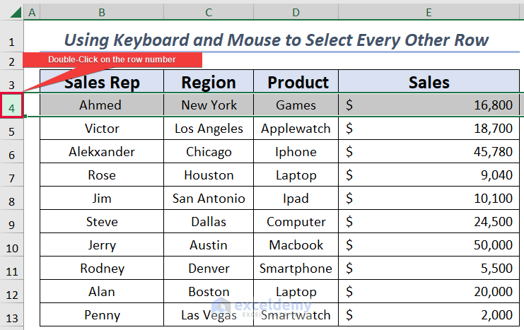
- It will select the Entire Row.
- Hold the CTRL key and select the rest of the rows of your choice using the right side of the mouse.
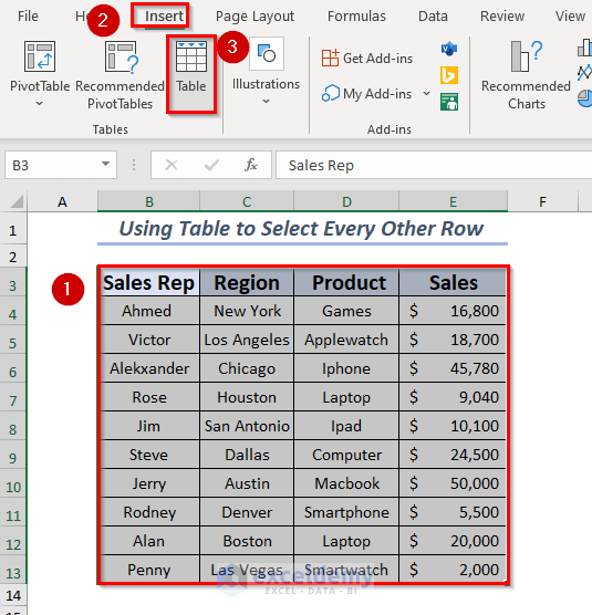
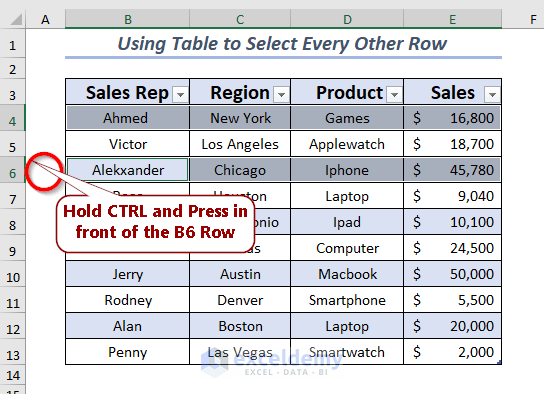
Method 4 – Utilizing Table Format
Steps:
- Select a range of rows to insert Table.
- Open the Insert tab >> select Table.
- A dialog box showing the selected range will pop up.
- Select My table has headers.
- Click OK.
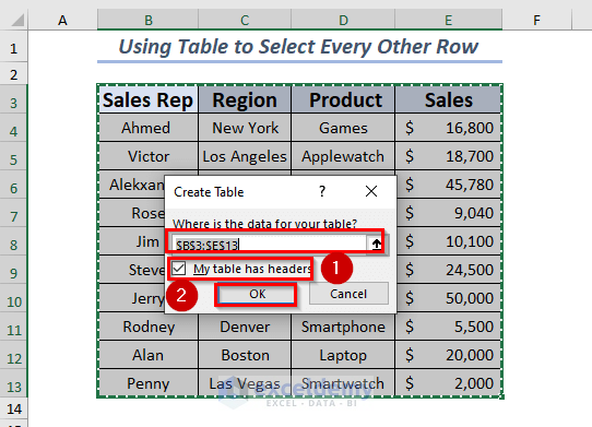
- The selected ranges will be converted into Table.
- Every other row has a different fill color to Highlight every other row.
- To select every other row of your choice, select any Highlighted row, hold the CTRL key, and select the rest of the Highlighted rows you want to select.
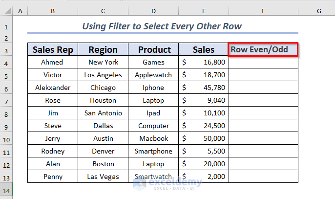
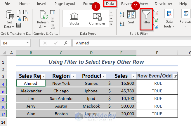
Method 5 – Using Filter with Go To Special
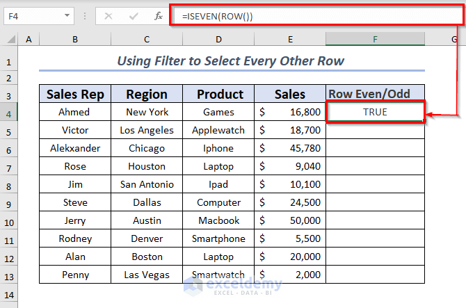
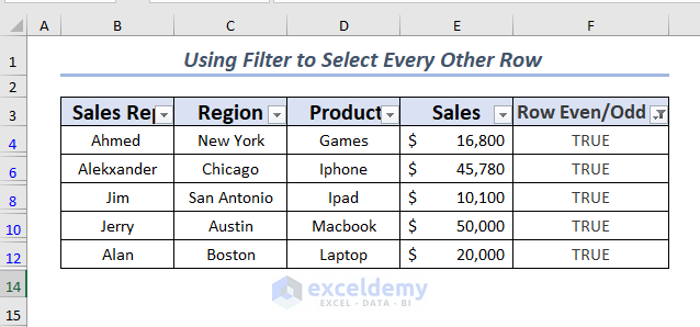
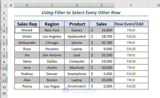
To select every other row using Filter with Go To Special, we added a new column in the dataset name Row Even/Odd. This column will show TRUE for even rows and False for odd rows.
Steps:
- Select the F4 cell and type the following formula,
=ISEVEN(ROW())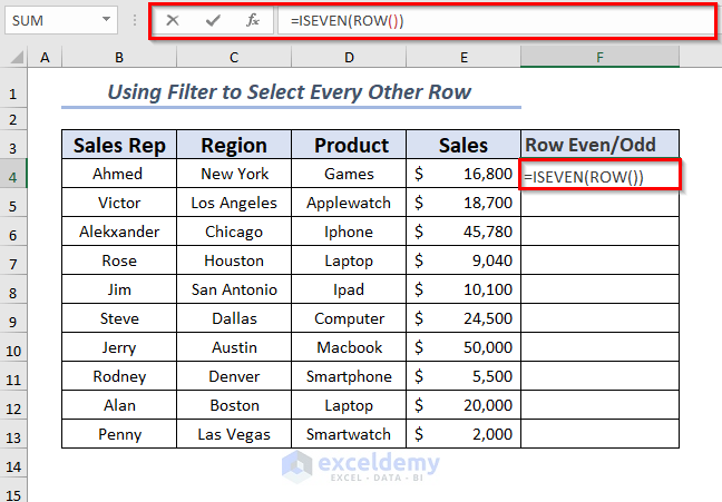
- Press Enter.
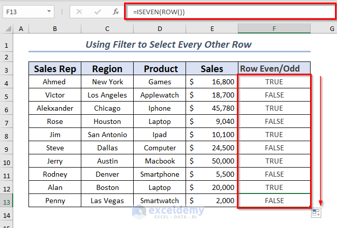
- It will show TRUE for row number 4 as it is an even number.
- Use the Fill Handle to AutoFill formula for the rest of the cells.
- Select the range where you want to apply the Filter.
- Select all the columns.
- Open the Data tab >> select Filter.
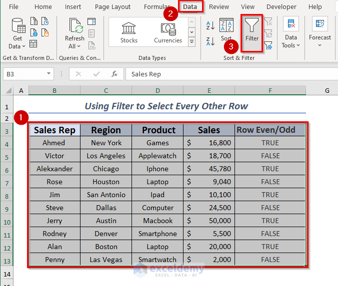
You also can use the CTRL+SHIFT+L keyboard shortcut.
- The Filter will be applied to all columns.
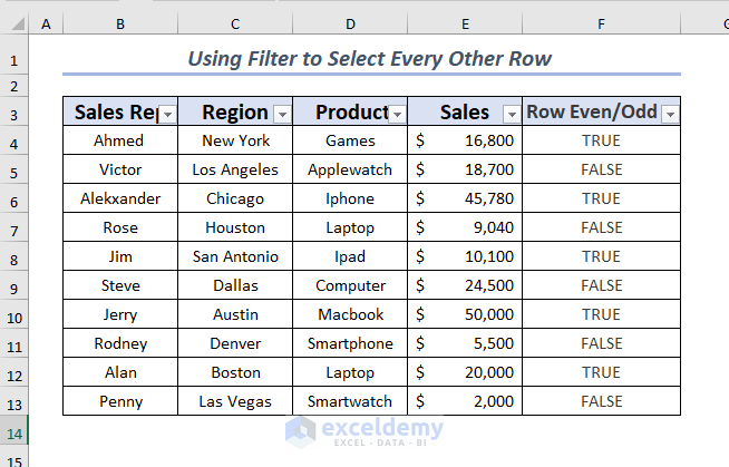
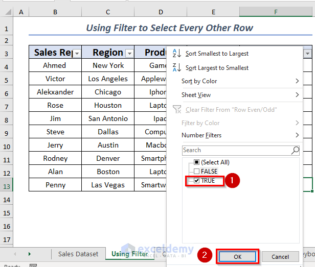
- Select the Row Odd/Even column to use Filter options.
- Select the TRUE value to Filter.
- Click OK.
- All the column values will be Filtered where the value is TRUE.
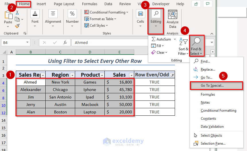
- Select the range where you want to apply Go To Special.
- Open the Home tab >> from Editing group >> Go to Find & Select >> select Go To Special
- A dialog box will be on the screen.
- Select the Visible cells only.
- Press OK.
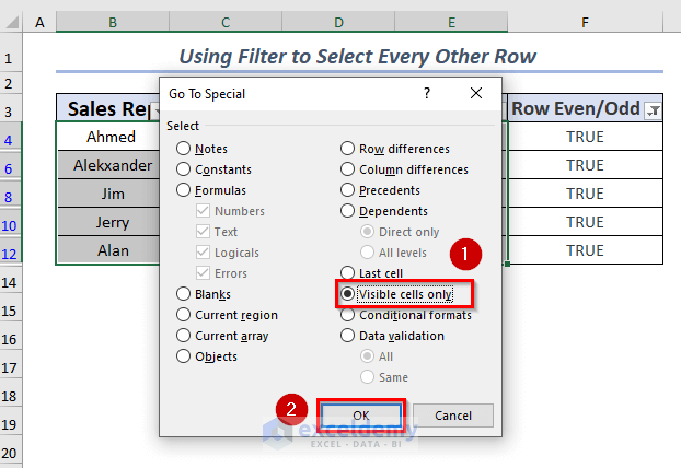
- The visible cells are selected.
- Open the Data tab >> select Filter.
- It will show the selected values along with all values by removing Filter.
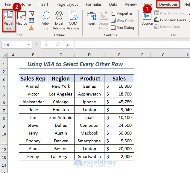
Method 6 – Applying VBA
Steps:
- Open the Developer tab >> select Visual Basic.
- A window for Microsoft Visual Basic for Applications will pop up.
- Click on Insert >> select Module.
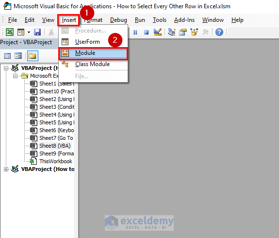
- A new Module will be opened.
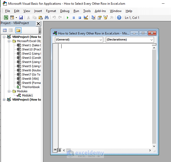
- Write the code to select every other row in the Module.
Sub SelectEveryOtherRow()
Dim userRange As Range
Dim OtherRowRange As Range
Dim rowCount, i As Long
Set userRange = Selection
rowCount = userRange.Rows.Count
With userRange
Set OtherRowRange = .Rows(1)
For i = 3 To rowCount Step 2
Set OtherRowRange = Union(OtherRowRange, .Rows(i))
Next i
End With
OtherRowRange.Select
End Sub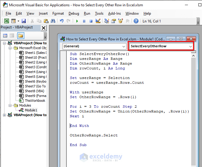
- Save the code and go back to the worksheet.
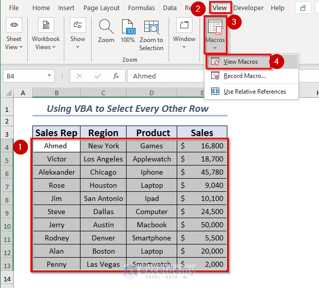
- Select the range where you want to apply the VBA.
- Open the View tab >> from Macros >> select View Macro.
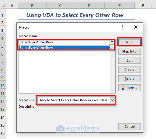
- A dialog box will pop up. Select the Macro name SelectEveryOtherRow.
- Click Run.
- Every other row will be selected from the first row.
Download Practice Workbook
Related Articles
- How to Select All Rows in Excel
- How Do I Quickly Select Thousands of Rows in Excel
- How To Select All Rows to Below in Excel
<< Go Back to Select Row | Rows in Excel | Learn Excel
Get FREE Advanced Excel Exercises with Solutions!

