Method 1 – Using the Format Axis Feature
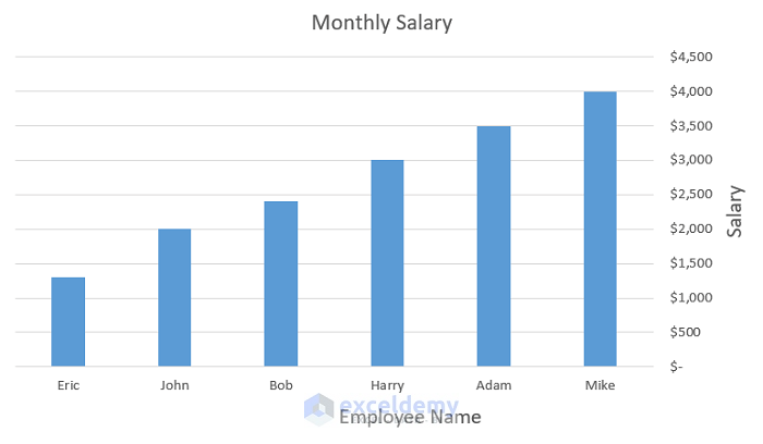
The sample dataset contains Employees’ Names and their respective Salary.
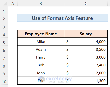
A Column Chart was created.
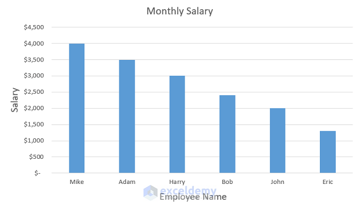
The X–axis represents the Employee Name, and the Y-axis represents the Salary.
To reverse the X-axis by using the Format Axis Feature:
Steps:
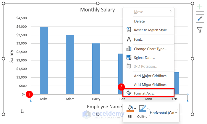
- Select the horizontal axis (i.e. X-axis) and right-click it.
- Select Format Axis.
- In the Format Axis dialog box, check Categories in reverse order.
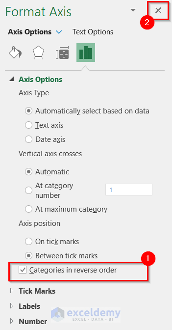
Note:
For Categories: check ‘Categories in reverse order’.
For Values: check ‘Values in reverse order’.
For Series in a 3-D chart: check ‘Series in reverse order’.
The X-axis is in reverse order.
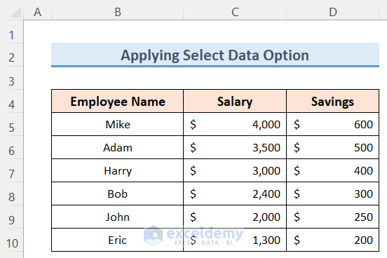
Method 2 – Applying the Select Data Option
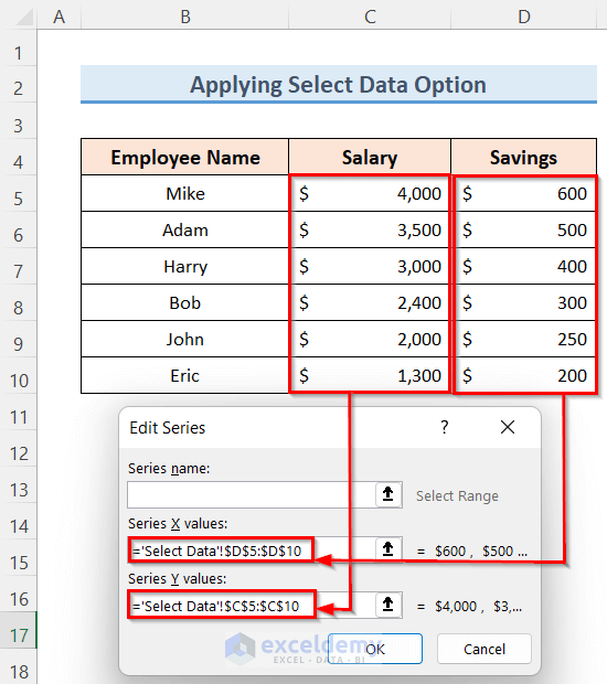
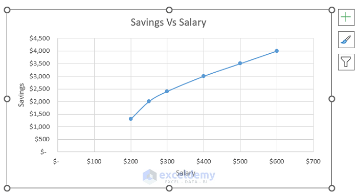
The following dataset showcases the Employee Name, Salary, and Savings over a period of time.
To reverse the X-axis to the Y–axis:
Steps:
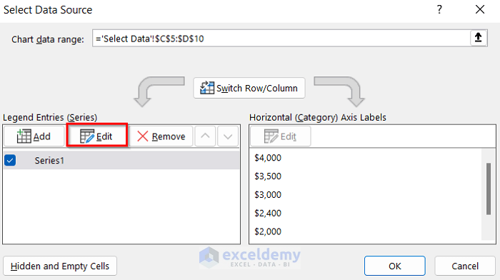
- Right-click the graph, and choose Select Data.
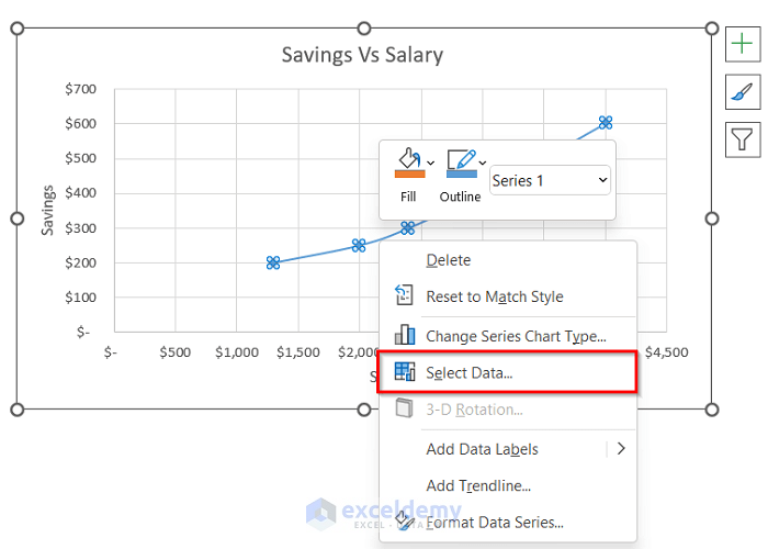
- In the Select Data Source dialog box, click Edit.
- In the Edit Series window Series X Values represent the Profit value range and Series Y Values represent the Salary.
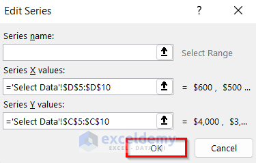
- Change the series: assign Salary to Series X Values and Profit to Series Y Values.
- Click OK.
- Click OK to close Select Data Source.
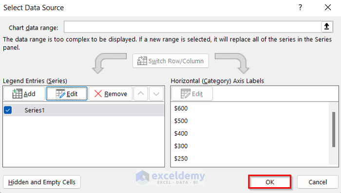
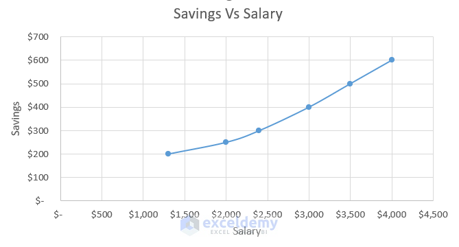
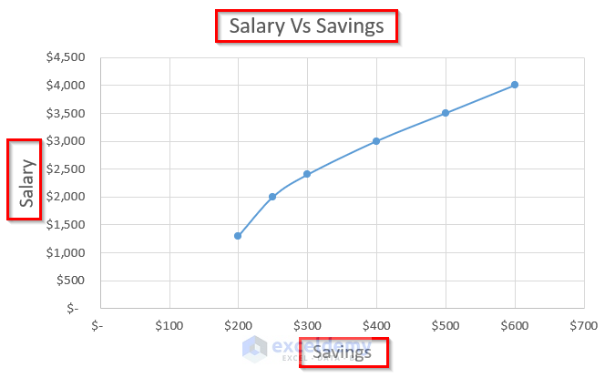
This is the output: the X and Y axes are reversed.
- Change the Axis Titles and the Chart Title.
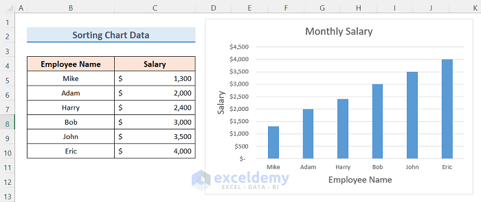
Method 3 – Sorting the Chart Data
This is the same dataset as in Method 1.
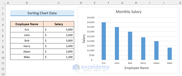
To reverse and arrange it in ascending order:
Steps:
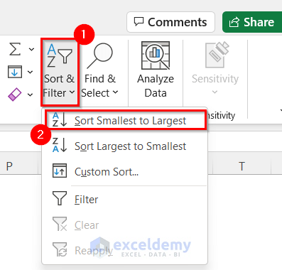
- Select (C5:C10) >> go to the Home tab.
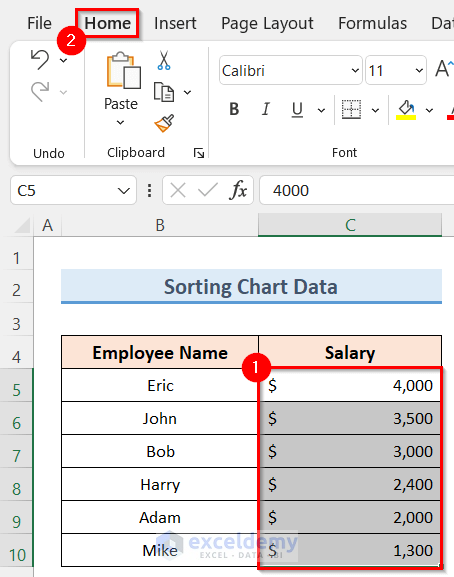
- Click Sort & Filter >> select Sort Smallest to Largest.
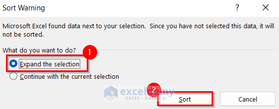
- In the Sort Warning dialog box, check ‘Expand the selection’ and click Sort.
- Both your chart data and the X-axis were reversed in ascending order.
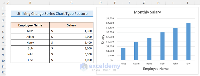
Method 4 – Utilizing the Change Series Chart Type Feature
To reverse the X axis with the ‘Change Series Chart Type feature’:
Steps:
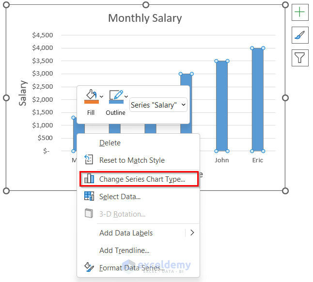
- Right-click any column in the chart.
- Select ‘Change Series Chart Type’.
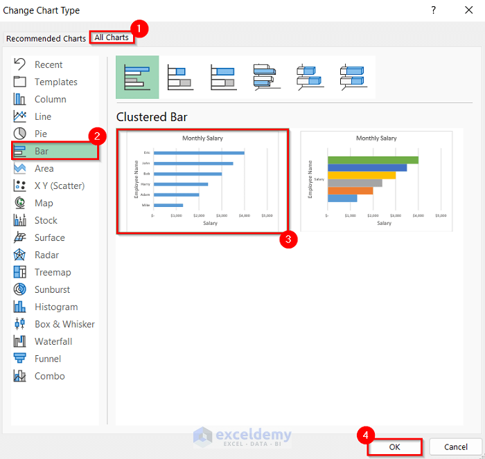
- In the Change Chart Type window, In All Charts, click Bar >> choose a Bar chart type (here Clustered Bar Chart type).
- Click OK.
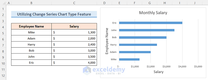
Your chart will change from column to Bar. The X-axis in the column chart is reversed to the Y-axis and vice versa.
Read More: Reverse X and Y Axis in Excel
Download Practice Workbook
Download the Excel workbook here.
<< Go Back To Format Axis in Excel | Excel Chart Elements | Excel Charts | Learn Excel
Get FREE Advanced Excel Exercises with Solutions!
