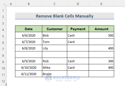
Here’s the overview of a sample dataset where blank cells are removed.
How to Remove Blank Cells in Excel: 10 Quick Ways
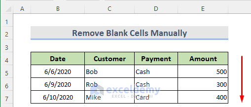
Method 1 – Removing Blank Cells Manually in Excel
We have a dataset of the Customer’s payment history with a lot of blank cells.
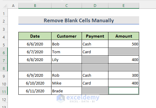
Steps:
- Select all the blank cells by holding the Ctrl key from the keyboard and clicking the cells.
- Right-click on the selection and choose Delete.
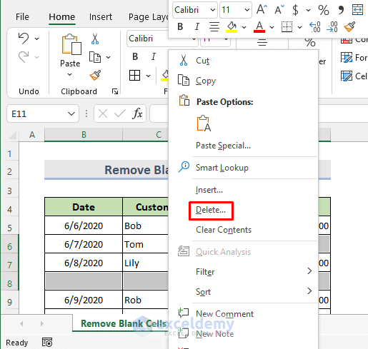
- Alternatively, go to Home and select Delete.
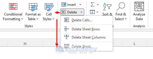
- Select an option and click OK.

- Here’s the result where entire rows with blank cells were removed.
Read More: How to Delete Blank Cells and Shift Data Up in Excel
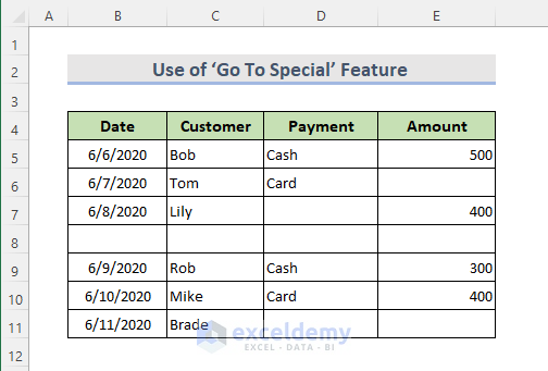
Method 2 – Using Go To Special to Delete Blank Cells
We have a payment history dataset.
Steps:
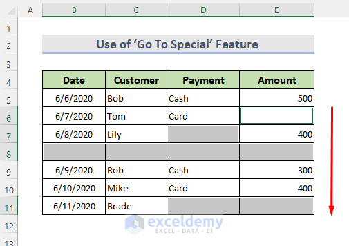
- Select the whole range containing blank cells.
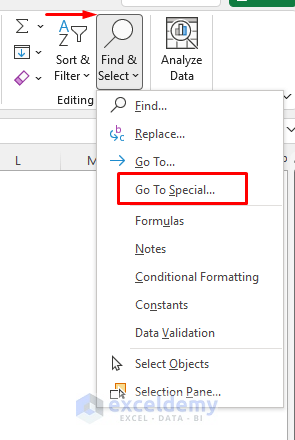
- Go to Home and, from the Find & Select drop-down, click Go To Special.
- Select the Blanks option and click OK.
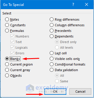
- Excel selects all blank cells.
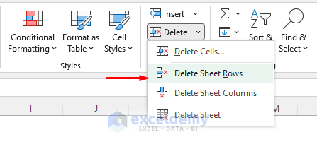
- Go to Home, choose Delete, and pick Delete Sheet Rows.
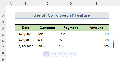
- Here’s the final result.
Read More: How to Remove Blank Cells from a Range in Excel
Method 3 – Use a Keyboard Shortcut to Erase Blank Cells in Excel
Steps:
- Select all the blank cells from the range.
- Press Ctrl + –.
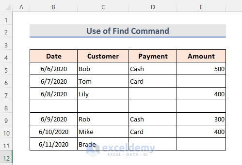
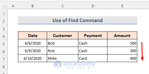
Method 4 – Remove Empty Cells with Find
We’ll use a similar dataset with some empty cells and rows.
Steps:
- Select the whole dataset.
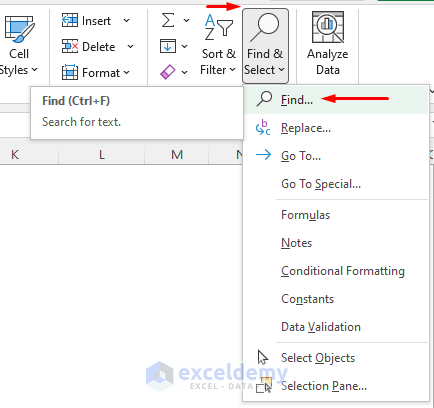
- In the Home tab, select Editing.
- Go to Find & Select and choose Find. You can also press the Ctrl + F keys to open the Find menu window.
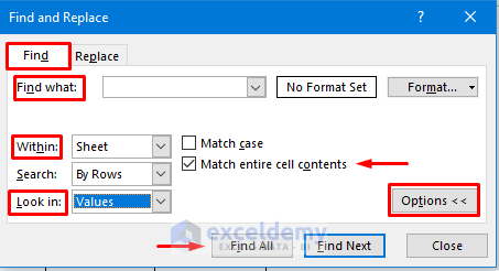
- Click Options to see the advanced search criteria.
- Keep the Find what box blank.
- Select Sheet from the Within the drop-down box.
- Make sure that the Match entire cell contents box is checked.
- Select Values from the Look in drop-down box.
- Click on Find All.
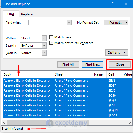
- You’ll get a result of the cells in the window below the settings.
- Press Ctrl + A to select all cells and click on Close.
- Go to Home, then select Delete and pick Delete Sheet Rows.

- Here’s the result.
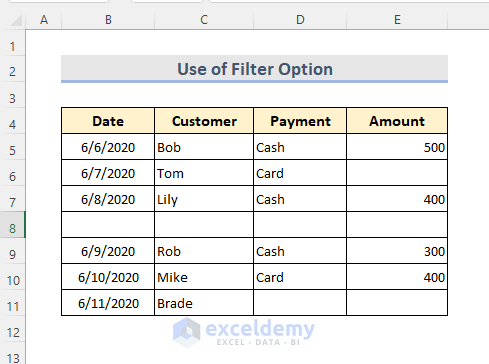
Method 5 – Use the Filter Option for Removing Blank Cells
We’ll use the same starting dataset.
Steps:
- Select the whole dataset.
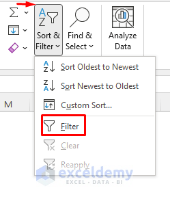
- Go to the Home tab.
- Click on Sort & Filter and pick Filter.
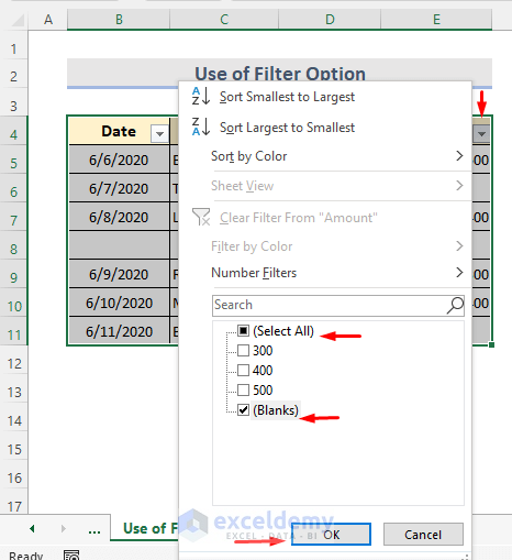
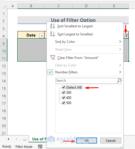
- You can see the filter toggle in each column. Select one of them.
- From the drop-down, uncheck Select All and check Blanks.
- Press OK.
- You can see the filtered blank cells.
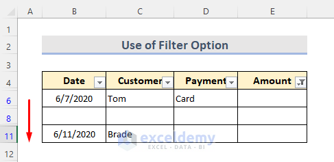
- Select the cells without the Header and delete them manually.
![]()
- Click on the filter toggle.
- Click on Select All and select OK.
- Here’s the filtered data without blank cells.
![]()
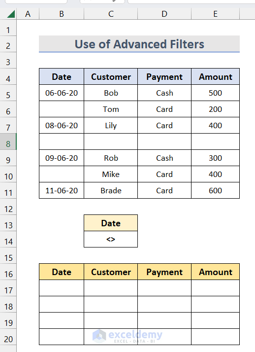
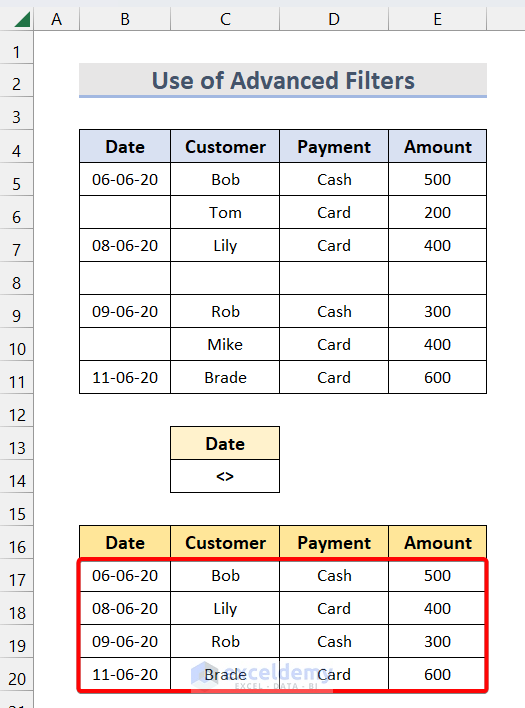
Method 6 – Use Advanced Filters to Remove Blank Cells in Excel
From the bellow dataset, we are going to remove all the blank Date cells.
- Select the criterion cell C14.
- Insert “<>”.
- Insert the table where you want to see the result.
- Select the original dataset.
- Go to Data and choose Advanced from Filter.
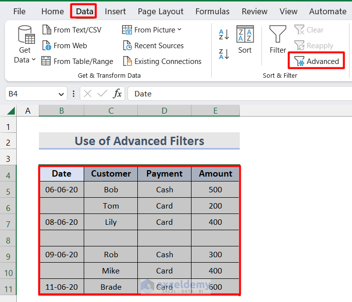
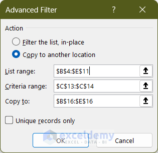
- A filter window pops up.
- Insert the list and criteria ranges, and where to copy.
- Select the option to copy to another location.
- Press OK.
- Here’s the result in the cell range B16:E16.
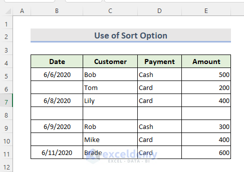
Method 7 – Use the Sort Option to Delete Excel Blank Cells
We have a dataset like in the previous methods.
Steps:
- Select the data range.
- Go to the Data tab.
- From the Sort & Filter section, select the ascending or descending Sort command.
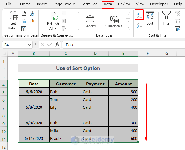
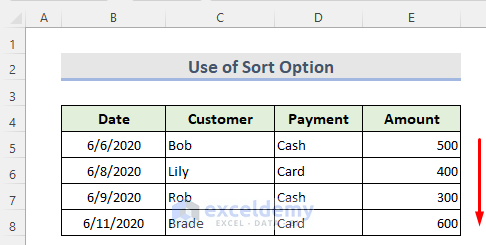
- All the blank cells are at the end of the dataset.
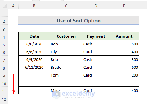
- Select the blank cells and delete them manually to see how the dataset looks.
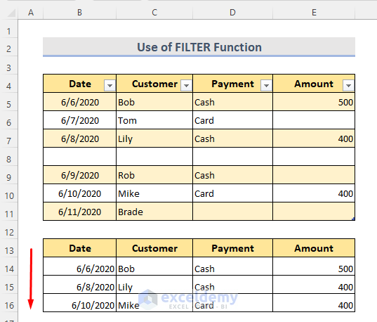
Method 8 – Using the FILTER Function to Remove Blank Excel Cells
We have a data table of the Customer’s payment history in the B4:E11 range. We are going to remove the blank cells and show the result in Cell B14 by filtering the data according to the Amount row.
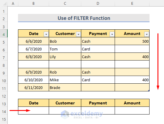
Steps:
- Select Cell B14.
- Insert the formula:
=FILTER(Table1,Table1[Amount]<>"","")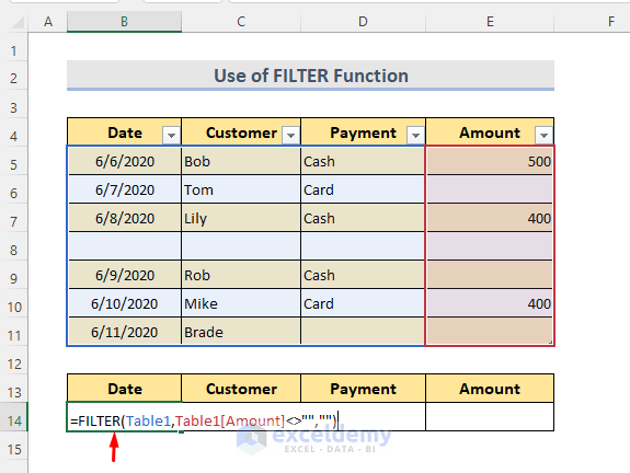
- Hit Enter to see the result.
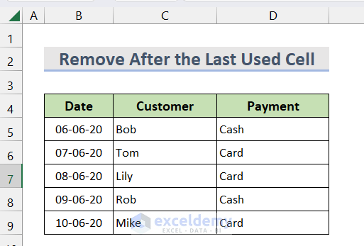
Method 9 – Erase Blank Cells After the Last Used Cell with Data
We have a few blank columns.
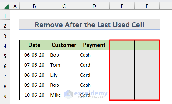
Steps:
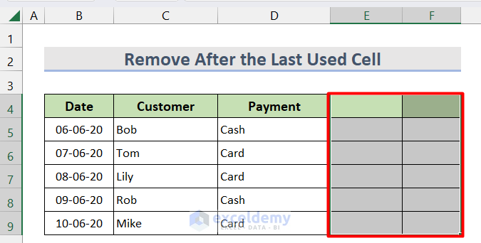
- Select the first blank cell.
- Press Ctrl + Shift + End.
- Go to Home, choose Delete, and pick Delete Sheet Columns.
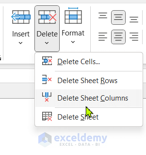
- You will see that the blank columns have been deleted.
Read More: How to Remove Unused Cells in Excel
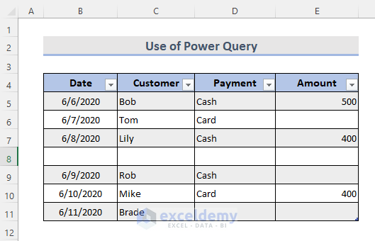
Method 10 – Using Power Query to Remove Empty Cells in Excel
Here is our data table.
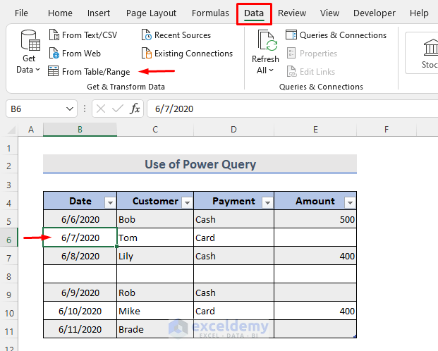
Steps:
- Select any cell in the table.
- Go to Data and select From Table/Range.
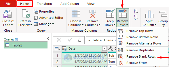
- Select the Home tab.
- From the Remove Rows drop-down, click Remove Blank Rows.
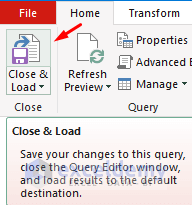
- Click the Close & Load option.
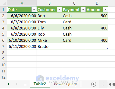
- You’ll get a table in a new worksheet.
Download the Practice Workbook
Excel Remove Blank Cells: Knowledge Hub
- How to Delete Blank Cells and Shift Data Up in Excel
- How to Remove Blank Lines in Excel
- How to Delete Blank Cells and Shift Data Left in Excel
- How to Remove Unused Cells in Excel
- How to Remove Blank Cells from a Range in Excel
<< Go Back to Excel Cells | Learn Excel
Get FREE Advanced Excel Exercises with Solutions!
