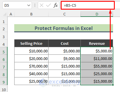
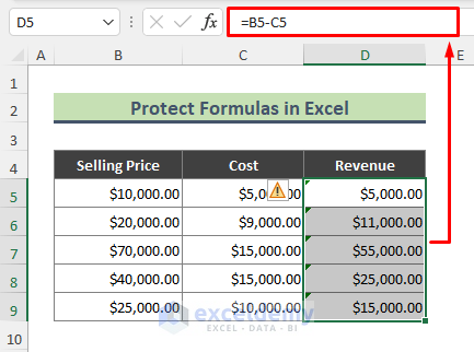
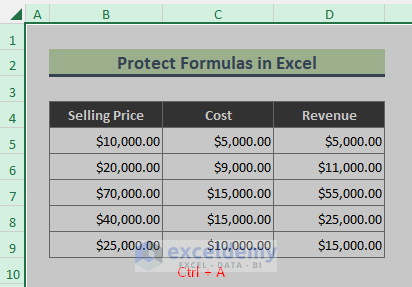
Dataset Overview
Suppose you have a dataset containing sales data, and you’ve used formulas to calculate revenues.
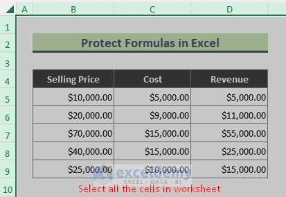
Step 1 – Unlock All Cells in the Excel Worksheet
- Select all the cells in the worksheet by pressing Ctrl + A.
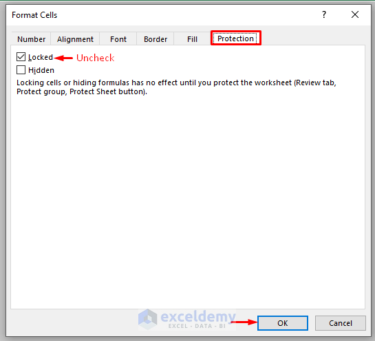
- Press Ctrl + 1 to open the Format Cells dialog (or right-click on the selection and choose Format Cells).
- In the Format Cells dialog, go to the Protection tab.
- Uncheck the Locked box option and press OK.
Read More: How to Protect Formulas Without Protecting Worksheet in Excel
Step 2 – Identify Cells Containing Formulas
- Select the entire worksheet by pressing Ctrl + A.
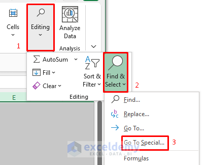
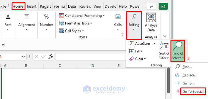
- From the Ribbon, go to the Home tab and find the Editing group.
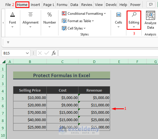
- Click on Find & Select and choose Go To Special.
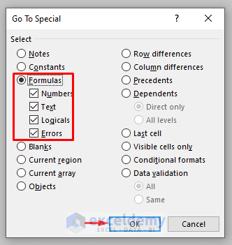
- In the Go To Special dialog, check the Formulas option and press OK.
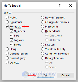
- All cells containing formulas will be highlighted.
Step 3 – Lock Only the Formula Cells
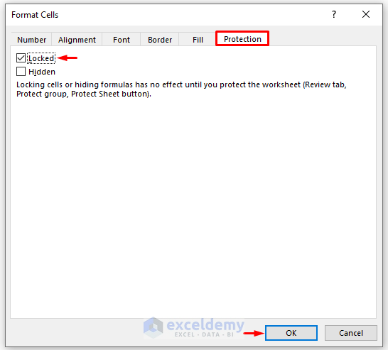
- While keeping the cells with formulas selected, press Ctrl + 1 to open the Formula Cells dialog.
- Under the Protection tab, check the Locked option and press OK. This will lock the formula cells again.
Step 4 – Protect Formulas in Excel
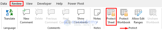
- Go to the Review tab and click on the Protect Sheet command.
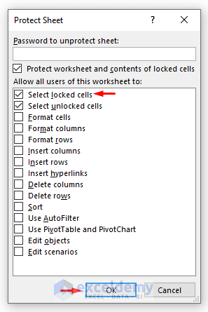
- The Protect Sheet dialog will appear.
- Make sure you’ve checked the Select locked cells option. Optionally, you can enter a password to unprotect the sheet.
- Press OK.
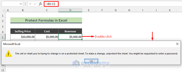
- Now all the formulas are protected. If you double-click any cell with formulas, Excel will display a warning indicating that you cannot edit the formulas.
Read More: How to Protect Formula in Excel but Allow Input
How to Hide Formulas in Excel for Protection
Sometimes, you might want to hide the formulas you’ve used in your calculations. Follow these steps:
Steps
- Select all the cells in the worksheet using Ctrl + A.
- Go to the Home tab, select Find & Select and choose Go To Special.
- In the Go To Special dialog, check Formulas and press OK.
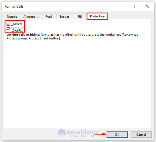
- Once you’ve found all cells with formulas, select them and use Ctrl + 1 to open the Format Cells dialog.
- Under the Protection tab, check both Locked and Hidden options, then press OK.
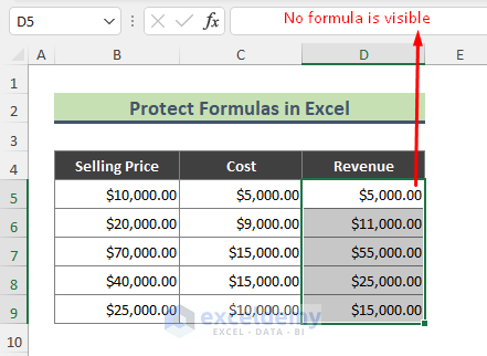
- Protect the sheet as explained in Step 4.
- After protecting the sheet, you’ll notice that the formulas are now hidden and locked.
How to Unprotect Sheet and Show Formulas in Excel
To unprotect formulas, follow these steps:
Steps:
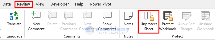
- Go to the Review tab and choose Unprotect Sheet.
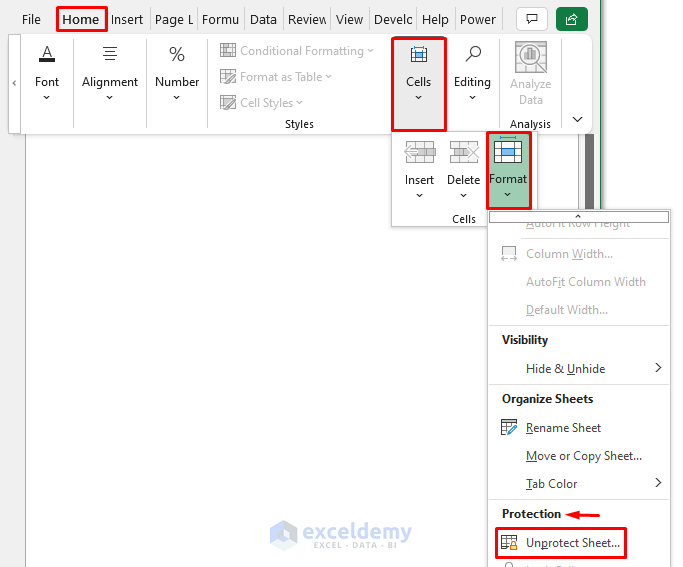
- Alternatively, from the Home tab, go to the Cells group, and select Format > Unprotect Sheet.
Adding the ‘Lock Cell’ Icon to the Excel Quick Access Toolbar
You can add the Lock Cell icon to the Quick Access Toolbar to easily check the status of cells. Here’s how:
Steps:
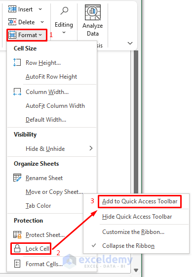
- Go to the Home tab.
- Click on Format and choose Lock Cell.
- Right-click on the Lock Cell icon and select Add to Quick Access Toolbar.
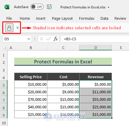
- The Lock Cell icon will now appear in the toolbar. When you select any locked cells, the icon will be shaded.
Download Practice Workbook
You can download the practice workbook from here:
Related Article
<< Go Back to Excel Formulas | Learn Excel
Get FREE Advanced Excel Exercises with Solutions!
