Method 1 – Using the Context Menu
Steps:
- Select all cells in the spreadsheet by clicking on the triangular sign where row headers and column headers meet.
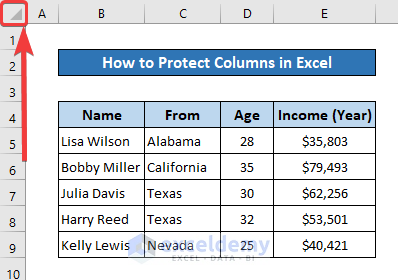
- Open the context menu by right-clicking on the selection or pressing Shift+F10.
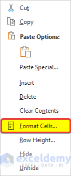
- Select Format Cells.
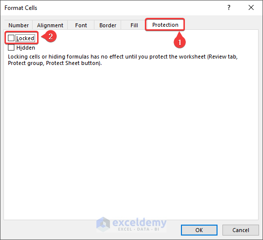
- Go to the Protection tab and uncheck the Locked option.
- Click on OK. This will unlock all the cells in the spreadsheet.
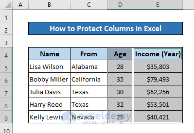
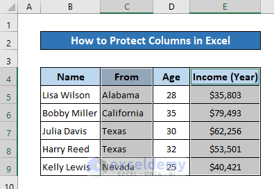
- Go back to your spreadsheet and select the columns you want to lock.
- Open the context menu. Select the Format Cells option.
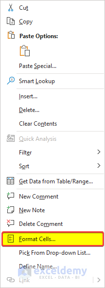
- Check the Locked option in the Protection tab from the Format Cells box.
- Click on OK.

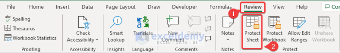
- Select the Review tab from your ribbon.
- Select Protect Sheet from the Protect group.
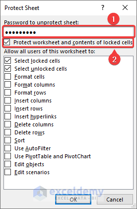
- A Protect Sheet box will appear. Here, make sure that the Protect worksheet and contents of locked cells option is checked.
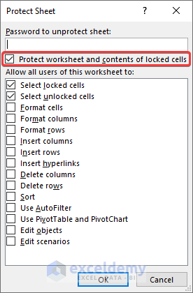
- Click on OK.
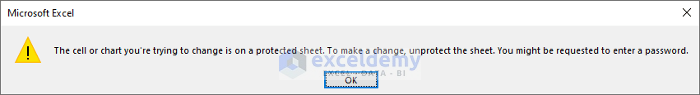
From now on, a warning box will appear, preventing the selected columns from being edited. You need to unprotect the sheet if you want to edit it further.
Method 2 – Using the Dialog Box Launcher
Steps:
- Click on the triangular sign where row headers and column headers meet to select all the cells in the spreadsheet.
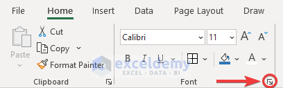
- Open the dialog box launcher by clicking on the downward-right facing arrow on the right of the group names in the Home tab.
- The Format Cells box will open. Go to the Protection tab and uncheck the Locked box.
- Click on OK.
- Select the columns you want to protect in the Excel spreadsheet.
- Open Format Cells. Check the Locked box from the Protection tab.
- Click on OK.
- Go to the Review tab.
- From the Protect group, select Protect Worksheet.
- To protect the columns with a password, enter one in the password field.
- Check that the Protect worksheet and contents of locked cells option is checked.
- Click on OK.
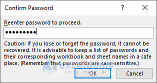
- If you entered a password in the previous box, a confirmation box will appear. Re-enter the password and click OK.
The selected columns will be locked, and a warning box will appear, preventing it from editing.
If you want to edit the protected columns again, you have to unprotect the sheet.
Method 3 – Applying the Format Cells Command
Steps:
- Select all the cells in the spreadsheet by clicking on the triangle sign where the row headers and column headers meet.
- Go to the Home tab.
- Click on Format from the Cells
- Select Format Cells from the drop-down menu.
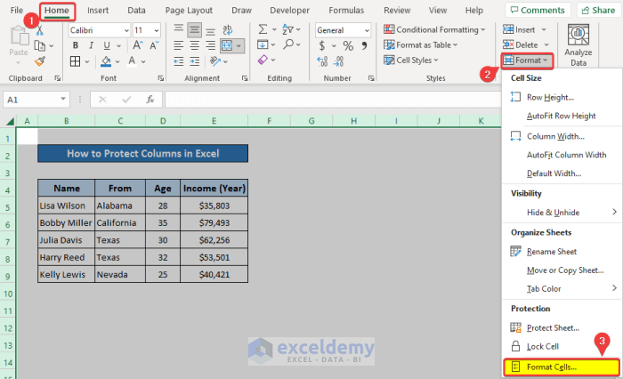
- The Format Cells box will appear. Go to the Protection tab and uncheck the Locked option.
- Click on OK.
- Select the columns you want to lock.
- Select Format from the Cells group in the Home tab and select the Format Cells option.
- Go to the Protection tab and check the Locked option.
- Click on OK.
- Go to the Review tab and select Protect Sheet from the Protect group.
- If you want to protect the columns with a password, check the Protect worksheet and contents of locked cells option and enter a password in the protection field.
- Click on OK.
This will protect all the columns in the Excel spreadsheet. If you want to edit any of the cells from the columns from now on, a warning box will appear, preventing the column from being edited.
Method 4 – Using Keyboard Shortcuts
Steps:
- Select all cells by clicking the triangle where all the row headers and column headers meet.
OR
- Click a blank cell in the Excel spreadsheet and press Ctrl+A.
- Press Ctrl+Shift+F or Ctrl+1 to open the Format Cells box.
- Go to the Protection tab and uncheck the Locked option.
- Click on OK.
- Select the columns you want to protect in the dataset.
- Press on the keyboard shortcuts again. Check the Locked option from the Protection tab in the Formula Cells box.
- Click on OK.
- Go to the Review tab.
- Select Protect Sheet from the Protect group.
- Check the Protect worksheet and contents of locked cells option in the Protect Sheet. Add a password in the password field if you want to protect the cells.
- Click on OK.
The locked columns are protected. If you try to edit any of the cells in those columns, a warning box will appear, preventing any form of change.
If you want to edit those columns, you need to unprotect the sheets and then edit those columns.
Method 5 – Using the ‘Allow Edit Ranges’ Feature
Steps:
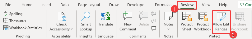
- Select the Review tab.
- Select Allow Edit Ranges from the Protect group.
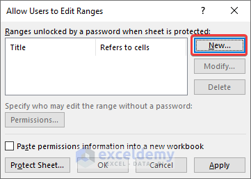
- A box called Allow Users to Edit Ranges will open. Select New.
- In the New Range box, select the range of cells in the Refers to cells.
- Add a title to the selected columns.
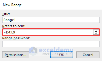
These are the columns you can edit in your spreadsheet.
- Click on OK.
- In the Allow Users to Edit Ranges box, select the range and then click on Protect Sheet.
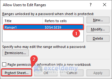
- Check the Protect worksheet and contents of locked cells option and click on OK.
After all the steps shown above, columns D and E will be editable, leaving all the cells, including columns B and C, protected from edits. If you want to edit anything in columns B and C, a warning box will appear, preventing you from editing the cells in the column.
Method 6 – Embedding VBA Code
Steps:
- Go to the Developer tab.
- Select Visual Basic from the Code group.
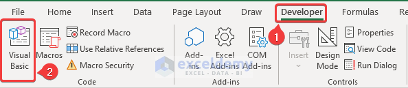
- The VBA window will open. Select the sheet from the left-hand side of the window.
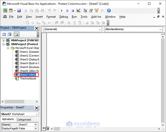
- Enter the following code in the VBA editor:
Private Sub Worksheet_SelectionChange(ByVal Target As Range)
Dim j As Integer

If Target.Column = 3 Then
For j = 5 To 9
If Target.Row = j Then
Beep
Cells(Target.Row, Target.Column).Offset(0, 1).Select
End If
Next j
End If

If Target.Column = 5 Then
For j = 5 To 9
If Target.Row = j Then
Beep
Cells(Target.Row, Target.Column).Offset(0, 1).Select
End If
Next j
End If
End Sub- Save and close the VBA window.
The code here is selected for columns C and E. We did that using column numbers. So if you want to edit columns C and E there will be a beep sound and the cell highlighter will automatically move to the right of the selection, preventing any edit in those columns.
Download the Practice Workbook
Download the workbook to practice.
Protect Columns in Excel: Knowledge Hub
<< Go Back to Excel Protect | Learn Excel
Get FREE Advanced Excel Exercises with Solutions!
