How to Protect Hidden Columns in Excel – 4 Methods

Method 1 – Using the Format Cells Command to Protect Hidden Columns

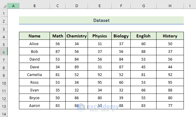
This is the sample dataset.

To hide columns:

Steps:

• Select column D.
• Press and hold Ctrl and select column G.

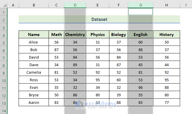
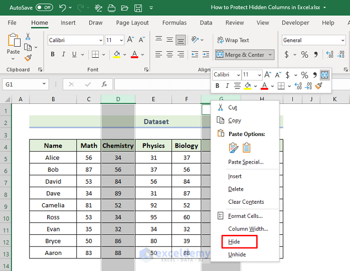
• Right-click the selected columns.
• In the context menu, select Hide.

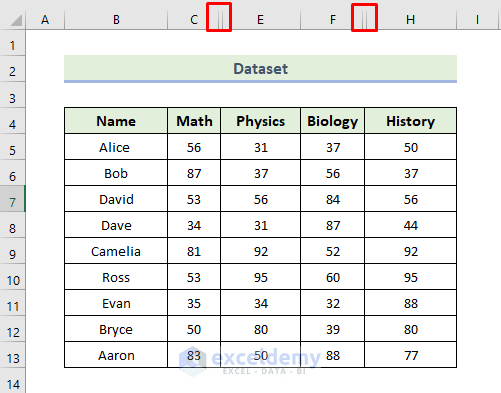
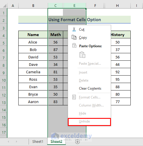
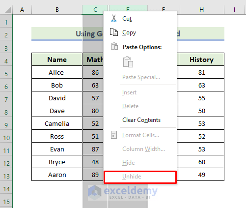
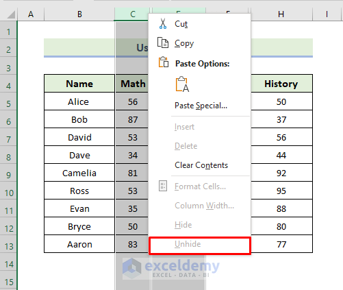
Columns D and G are not displayed.

To protect the hidden columns:

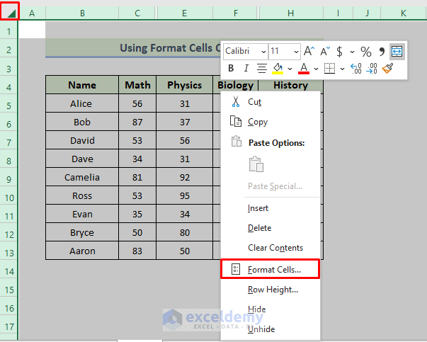
• Select the whole sheet, right-click and select Format Cells.

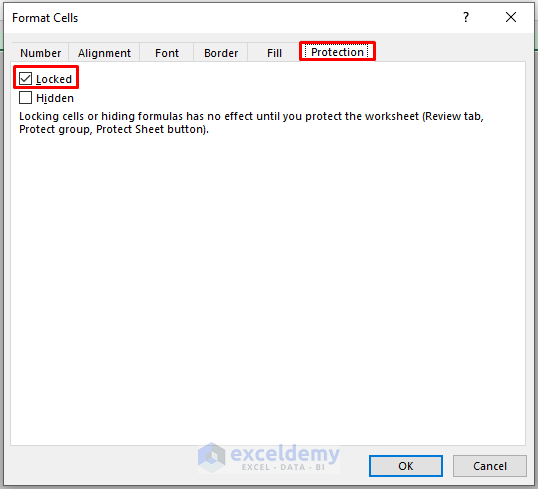
• In the Format Cells dialog box, select Protection.
• Check Locked.
• Click OK.

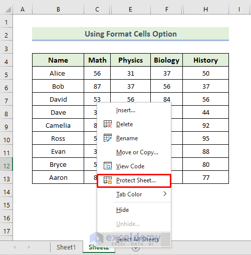
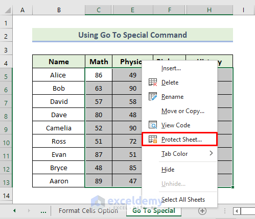
• Place the cursor on the active sheet name, right-click and select Protect Sheet.

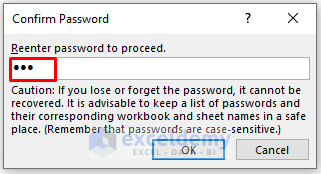
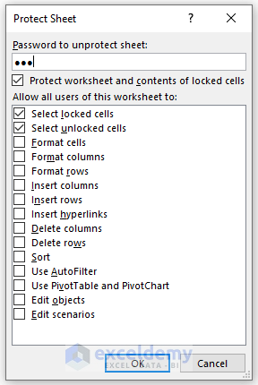
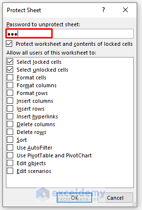
• In the Protect Sheet dialog box, enter a the password.
• Click OK.

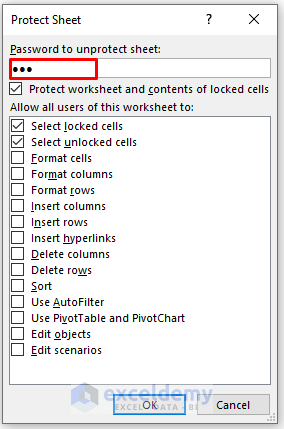
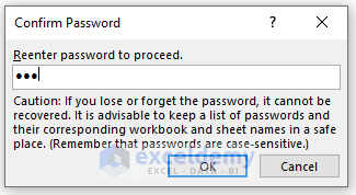
• To confirm, enter the password again and click OK.

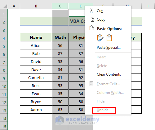
The hidden columns are protected.

Method 2 – Using the Go To Special Command to Protect Hidden Columns in Excel

Steps:

• Select column D.
• Press and hold Ctrl and select column G.

• Right-click the selected columns.
• In the context menu, select Hide.

Columns D and G are not displayed.

To Protect the hidden columns:

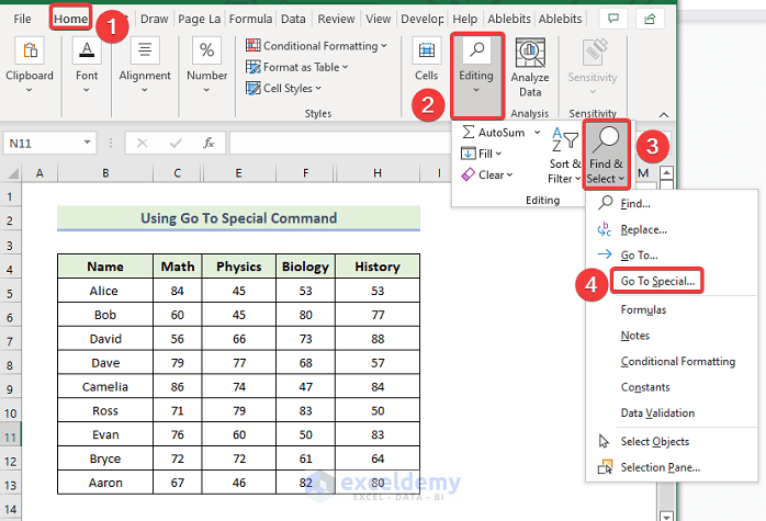
• Go to the Home tab, select Editing.
• Choose Find & Select.
• Select Go To Special.

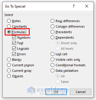
• Select Formulas and click OK.

• Place the cursor on the active sheet name, right-click and select Protect Sheet.

• In the Protect Sheet dialog box, enter a the password.
• Click OK.

• Enter the password again and click OK.

The hidden columns are protected.

Method 3 – Using the Info Option to Protect Hidden Columns

Steps:

• Select column D.
• Press and hold Ctrl and select column G.

• Right-click the selected columns.
• In the context menu, select Hide.

Columns D and G are not displayed.

To protect the hidden columns:

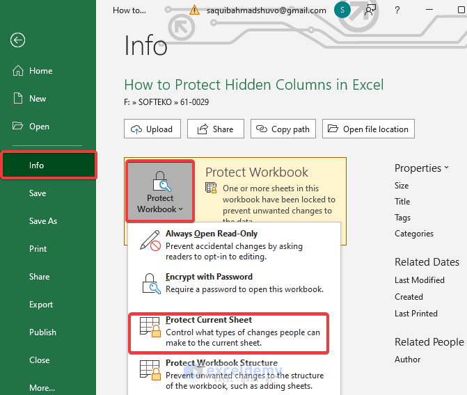
• Go to the File tab.

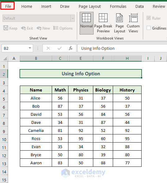
• Select Info, and choose Protect Workbook.
• Select Protect Current Sheet.

• In the Protect Sheet dialog box, enter a password.
• Click OK.

• Enter the password again and click OK.

The hidden columns are protected.

Read More: How to Protect Columns with Password in Excel

Method 4 – Embedding a VBA Code to Protect Hidden Columns

 Steps:

• Select column D.
• Press and hold Ctrl and select column G.

• Right-click the selected columns.
• In the context menu, select Hide.

Columns D and G are not displayed.

Use a VBA code to protect the hidden columns.

• Press Alt+F11 to open the VBA editor. Select Insert > Module.

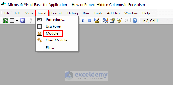
• Enter the following code in the module.

Sub Protect_Hidden_Columns()
Dim HPassword As String
Range("B5:H13").Select
Selection.Locked = True
HPassword = InputBox("Type Password to Protect Hidden Columns")
ActiveSheet.Protect Password:=HPassword
End Sub

• Close the Visual Basic window.
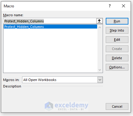
• Press Alt+F8.
• In the Macro dialog box opens, select Protect_Hidden_Columns in Macro name.
• Click Run.

• Enter a password to protect the hidden columns.

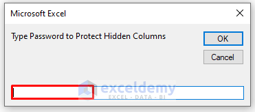
The hidden columns are protected.

Download Practice Workbook

Download the practice workbook.

<< Go Back to Protect Excel Columns | Excel Protect | Learn Excel