How to Create Non-GST Invoice Format in Excel (5 Steps)

Step 1 – Make Outline of Non-GST Invoice Format in Excel

• Begin by setting up the basic inputs. You’ll need a Product List in one sheet and a Customer List in another. Here’s what each list should contain:
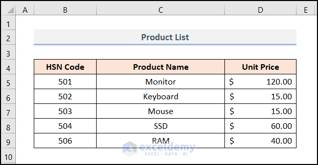
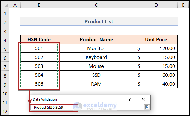
  • Product List (Columns B, C, and D):
    • HSN Code of the products
    • Product Name
    • Unit Price
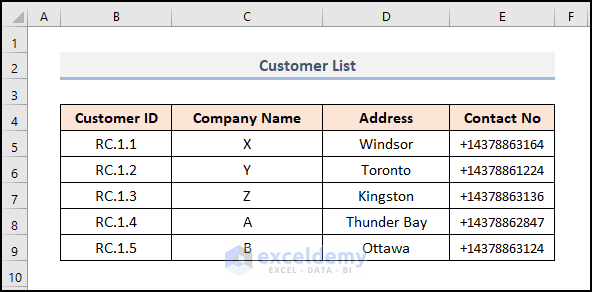
  • Customer List:
    • Customer ID
    • Company Name
    • Address
    • Contact No.

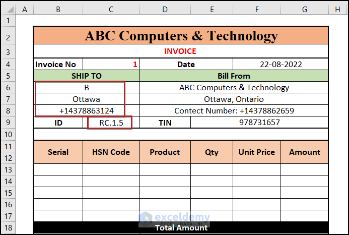
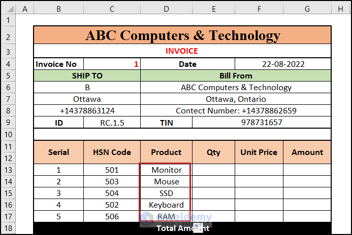
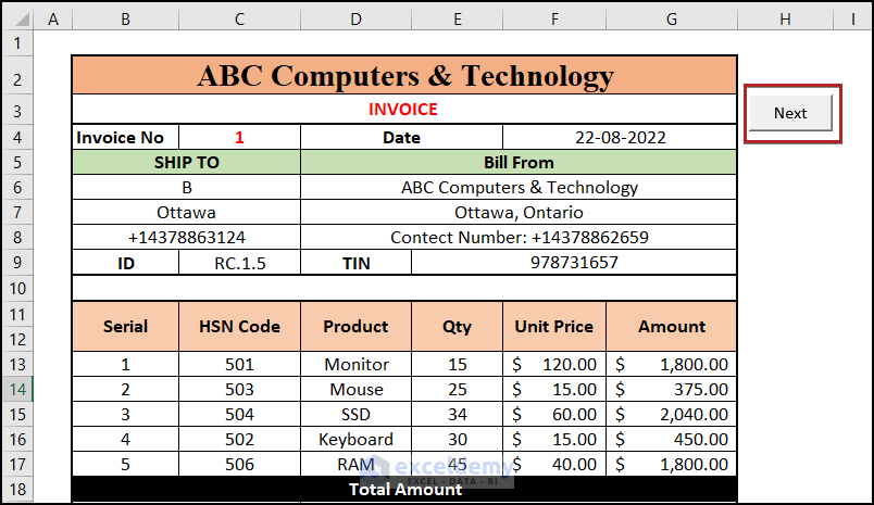
• Create the necessary outline for the non-GST invoice. enter the company’s address and contact number in cells D6:D8. Additionally, put the TIN number in cell E9.

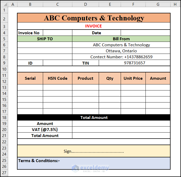
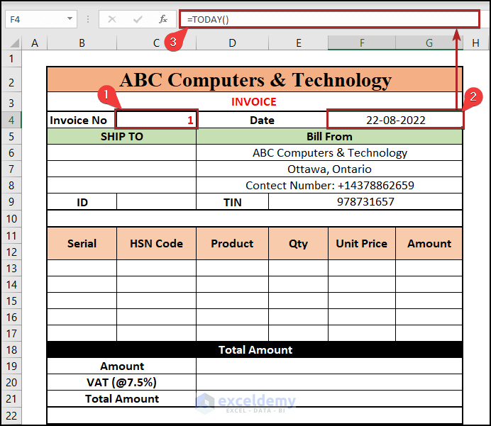
• In cell C4, enter 1 as the Invoice No since it’s our first invoice.
• Select cell F4 and enter the following formula in the Formula Bar:

The Today function returns the current date.

• Press ENTER.

Read More: How to Create a Tally GST Invoice Format in Excel

Step 2 – Create a Drop-down List

• To easily select values for the invoice, create a dropdown list of the ID numbers of the companies you’ll be supplying products to.
• Select cell C9 where you want the dropdown list.
• Go to the Data tab and choose Data Validation in the Data Tools group.

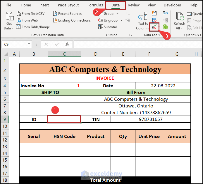
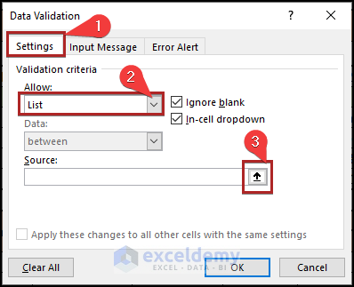
• In the Data Validation dialog box, move to the Settings tab.
• Select List from the dropdown list in the Allow section.
• Click the upside arrow next to the Source box to open the Data Validation input box.

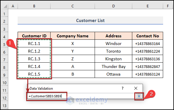
• Select cells B5:B9 in the Customer worksheet.
• Click the down-side arrow to return to the Data Validation dialog box.

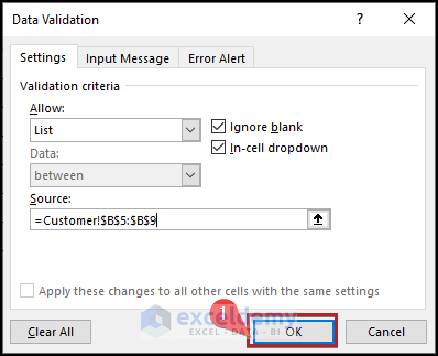
• Finally, click OK to create the dropdown list.

• Test it by selecting cell C9 and clicking the dropdown arrow icon.
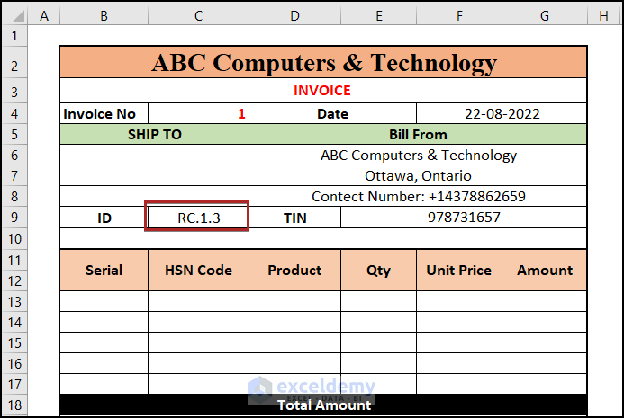
• Choose R.C.1.3 from the list to see the Customer ID in the cell.

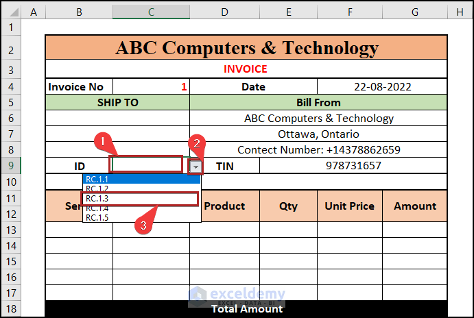
• We can see the Customer ID in our cell.

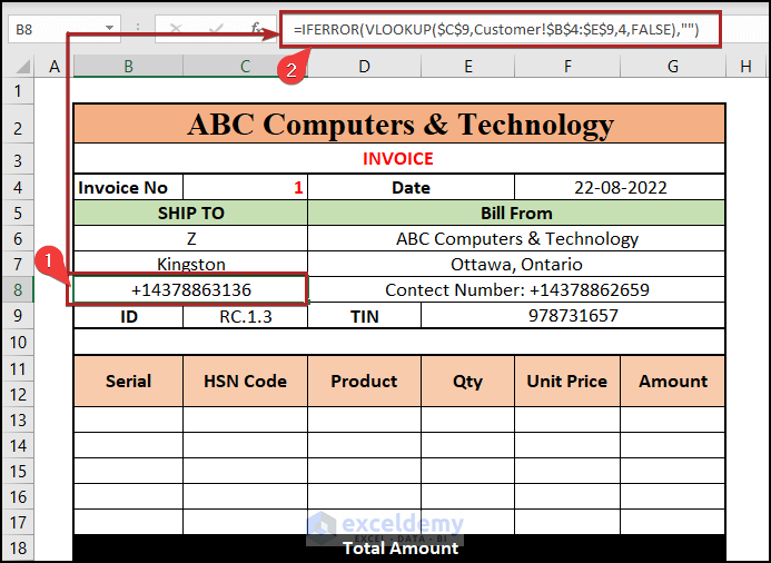
Step 3 – Acquire Shipping Details

Company Name Lookup:

• Select cell B6.
• Enter the formula below:

Here:

• • $C$9 is the lookup value (the specific ID).
  • Customer!$B$4:$E$9 is the table array (Customer sheet).
  • 2 represents the column number for Company Name.
  • FALSE ensures an exact match.
• If VLOOKUP returns an error, the IFERROR function converts it to a blank cell.
• Press ENTER. You’ll see the Company Name (e.g., Company A) for the specific ID R.C.1.3.

Address and Contact No Lookup:

• Similarly, enter these formulas for Address and Contact No:

• Now you have the corresponding Company Name, Address, and Contact No for the ID R.C.1.3.

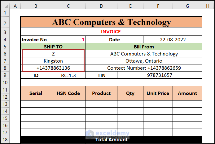
• Changing the ID via the dropdown list will update these details.

Read More: How to Make GST Export Invoice Format in Excel

Step 4 – Modify Non-GST Invoice Format

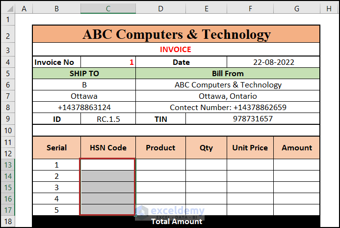
• Dropdown Lists for Product Codes:
  • Create dropdown lists for cells C13:C17 (similar to Step 2).

• • Use cells B5:B9 in the Product sheet as the source.

• We successfully created the dropdown list in these cells.
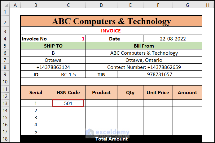
• For testing purposes, select cell C13 and click on the dropdown arrow icon.
• Select 501 from the list.

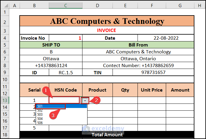
• The selected HSN Code will appear in cell C13.

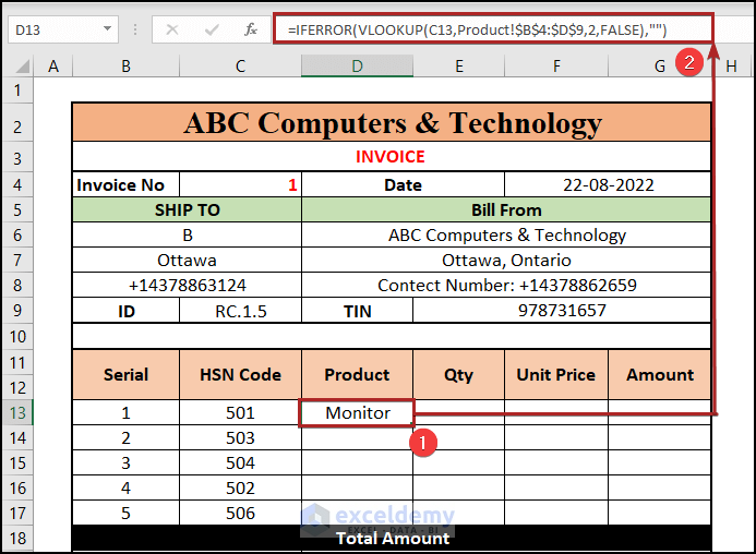
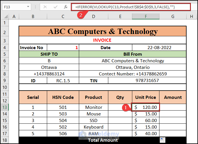
• Product Name Lookup:
  • In cell D13, enter:

• • • This retrieves the Product Name based on the selected HSN Code.
  • Press ENTER.

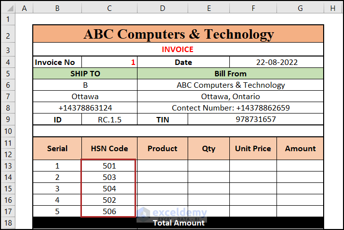
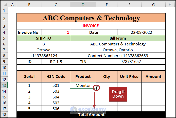
• Drag down the Fill Handle to fill D13:D17 with Product Names.

• We’ll get the Product Names in the Product column.

• Unit Price Calculation:
  • In cell F13, enter:

• • • This gets the Unit Price.
  • Press ENTER.

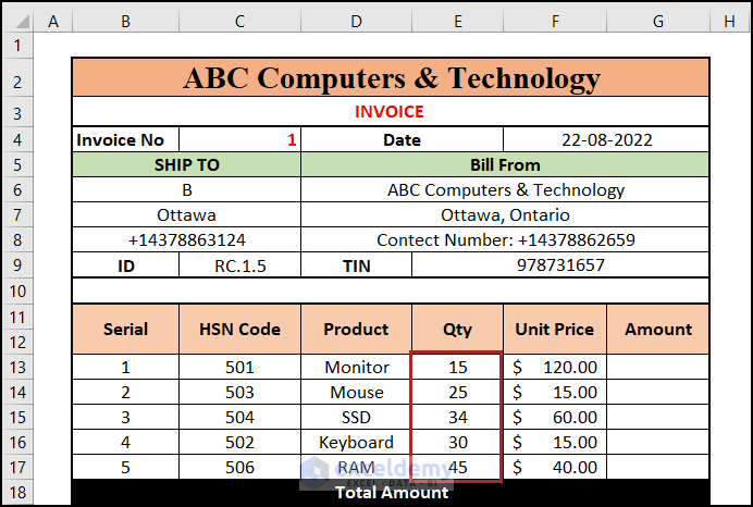
• • Enter the respective quantities in the Qty column (column E).

• • In cell G13, calculate the amount:

• • Press ENTER.

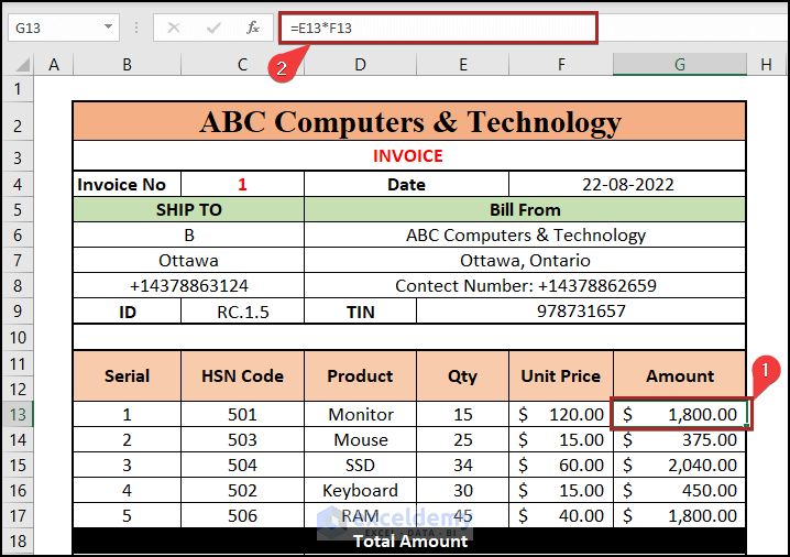
Note: Here, it multiplies the quantity with the unit price to get the amount.

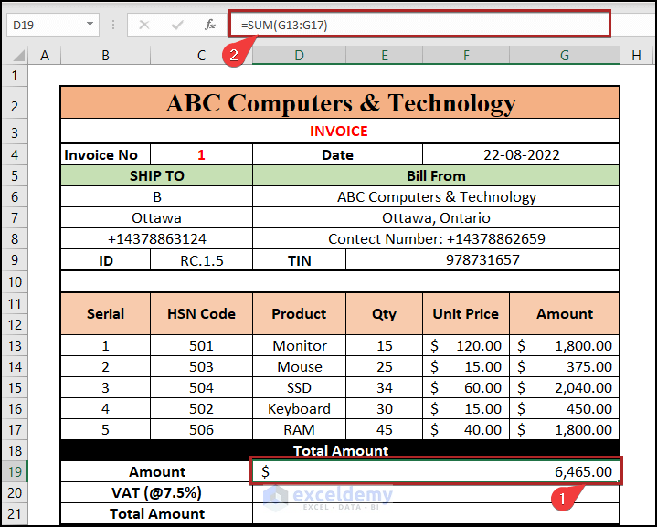
• Total Amount and VAT:
  • In cell D19, sum the amounts (G13:G17):

• • Press ENTER.

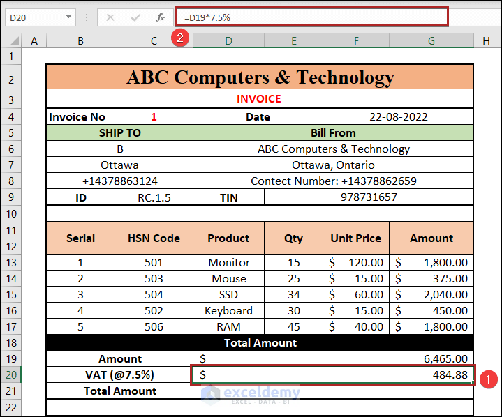
• • For VAT (7.5%), use cell D20:

• • Press ENTER.

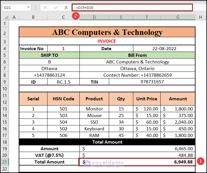
• • Finally, calculate the Total Amount in cell D21:

• • Press ENTER.

Read More: How to Create Proforma Invoice for Advance Payment in Excel

Step 5 – Save and Resume Invoice in Excel

Refresh the Invoice Form:

• Open the Developer tab. If it’s not visible, follow the instructions to display it on the ribbon.
• Select Visual Basic in the Code group or press ALT+F11.

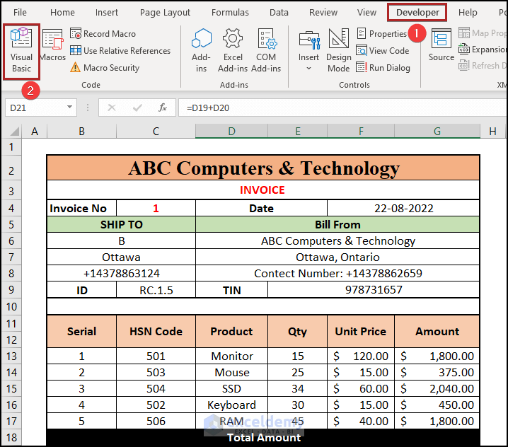
• The Microsoft Visual Basic for Applications window will open.
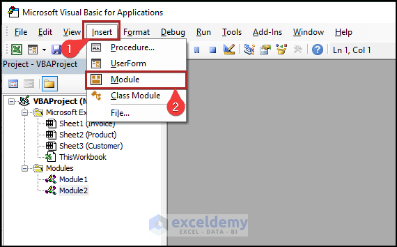
• Move to the Insert tab and choose Module.

• In the Code Module, enter the following code to go to the next invoice:

Sub next_invoice()
Range("C4").Value = Range("C4").Value + 1
Range("C13:C17").ClearContents
Range("E13:E17").ClearContents
Range("C9").ClearContents
End Sub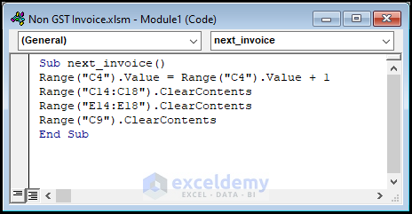

• Repeat the steps to create another module.
• In the new module, write this code to save the invoice:

Sub save_invoice()
Set ws = Worksheets("Invoice")
ws.Range("A1:G27").ExportAsFixedFormat xlTypePDF, _
Filename:="Invoice" & ws.Range("C4").Value, _
openafterpublish:=False
End Sub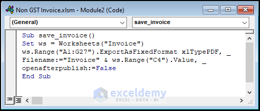

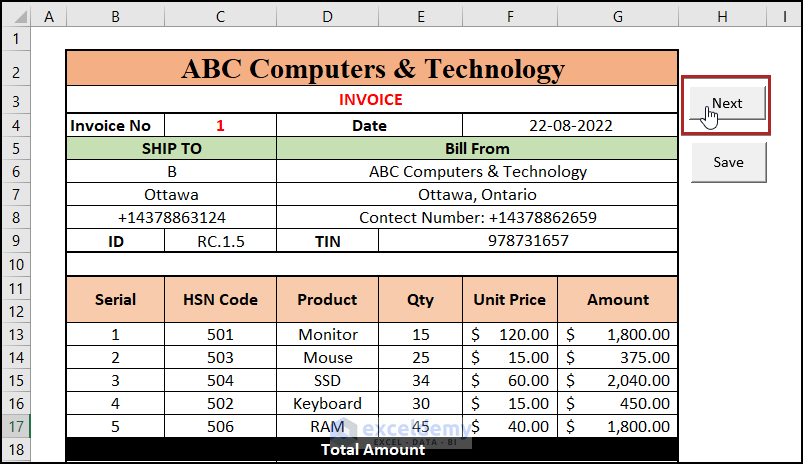
• Create Buttons for Next and Save:
  • Return to the Invoice worksheet.
  • Go to the Developer tab again.
  • Click Insert in the Controls group.
  • Choose Button under the Form Controls section.

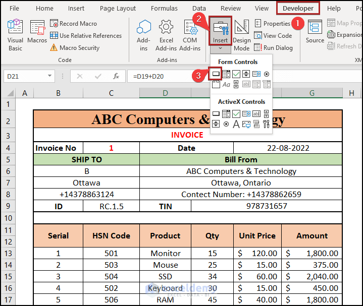
• Create a button in the designated region (as shown in the image). Name it Next.

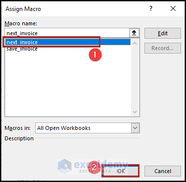
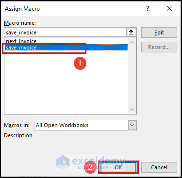
• Right-click the button and select Assign Macro.

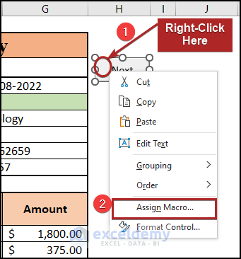
• Assign the macro next_invoice.

• Similarly, create another button named Save.

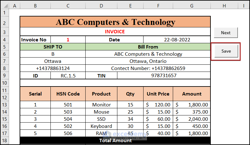
• Assign the macro save_invoice to the Save button.

• Save as PDF:
  • Click the Save button. The invoice will be saved as a PDF.

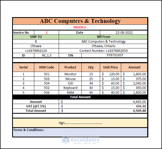
• Note: The image you see is the saved PDF version of Invoice No. 1.

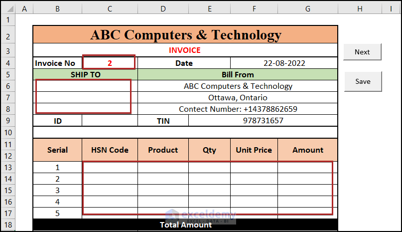
• Click the Next button to automatically set the Invoice No. to 2 and clear the values in the highlighted cells.

Read More: Proforma Invoice Format in Excel with GST

Download Practice Files

You can download the practice workbook from here:

Related Articles

• How to Create GST Rental Invoice Format in Excel
• Tally Sales Invoice Format in Excel
• How to Create GST Bill Format in Excel with Formula

<< Go Back to Excel Invoice Templates | Accounting Templates | Excel Templates