Method 1 – Use of Combined Functions to Mirror Text in Excel
Steps:
- Select Cell C5.
- Insert the following formula.
=TEXTJOIN("",1,MID(B5,ABS(ROW(INDIRECT("1:"&LEN(B5)))-(LEN(B5)+1)),1))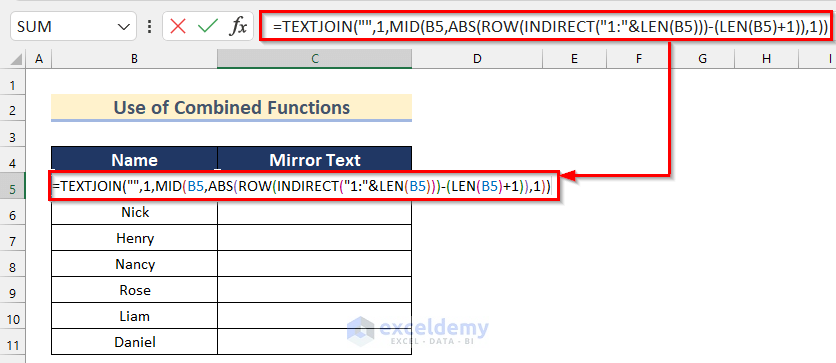
Formula Breakdown
- LEN(B5)—–> The LEN function returns the length of a text.
- Output: {5}
- ROW(INDIRECT(“1:”&LEN(B5)))—–>The ROW function returns the row number of a given Cell.
- ROW(INDIRECT(“1:”&5))—–> turns into
- Output: {1;2;3;4;5}
- ROW(INDIRECT(“1:”&5))—–> turns into
- ABS(ROW(INDIRECT(“1:”&LEN(B5)))-(LEN(B5)+1))—–> The ABS function returns the absolute value of a number.
- ABS({1;2;3;4;5}-(5+1))—–> becomes
- Output: {5;4;3;2;1}
- ABS({1;2;3;4;5}-(5+1))—–> becomes
- MID(B5,ABS(ROW(INDIRECT(“1:”&LEN(B5)))-(LEN(B5)+1)),1)—–> The MID function returns a number of strings from a given middle string.
- MID(B5,{5;4;3;2;1},1)—–> turns into
- Output: {“y”;”l”;”i”;”m”;”E”}
- MID(B5,{5;4;3;2;1},1)—–> turns into
- TEXTJOIN(“”,1,MID(B5,ABS(ROW(INDIRECT(“1:”&LEN(B5)))-(LEN(B5)+1)),1))—–> The TEXTJOIN function returns the joined string value.
- TEXTJOIN(“”,1,{“y”;”l”;”i”;”m”;”E”})—–> turns into
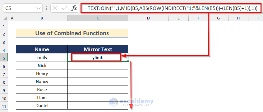
- Output: {ylimE}
- TEXTJOIN(“”,1,{“y”;”l”;”i”;”m”;”E”})—–> turns into
- Press ENTER to get the value of Mirror Text.
- Drag down the Fill Handle tool to AutoFill the formula for the rest of the cells.
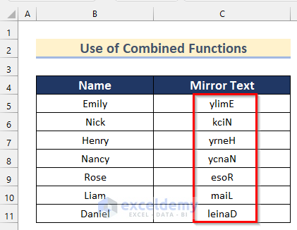
- Get all the Mirror Text values.
Method 2 – Using CONCATENATE and TRANSPOSE Functions to Mirror Text
Steps:
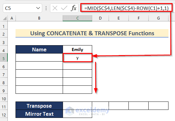
- Select Cell C5.
- Insert the following formula.
=MID($C$4,LEN($C$4)-ROW(C1)+1,1)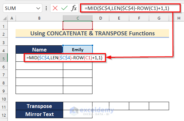
Formula Breakdown
- LEN($C$4)—–> The LEN function returns the length of a text.
- Output: {5}
- ROW(C1)—–> The ROW function returns the row number of a given Cell.
- Output: {1}
- MID($C$4,LEN($C$4)-ROW(C1)+1,1)—–> The MID function returns a number of strings from a given middle string.
- MID($C$4,5-{1}+1,1)—–> turns into
- Output: {“y”}
- MID($C$4,5-{1}+1,1)—–> turns into
- Press ENTER to get the last letter.
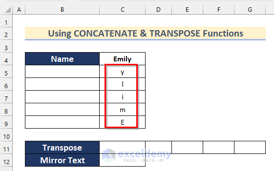
- Drag down the Fill Handle tool to AutoFill the formula for the rest of the cells.
- Get all the letters of the text in mirror form.
- Select Cell C11.
- Insert the following formula.
=TRANSPOSE(C5:C9)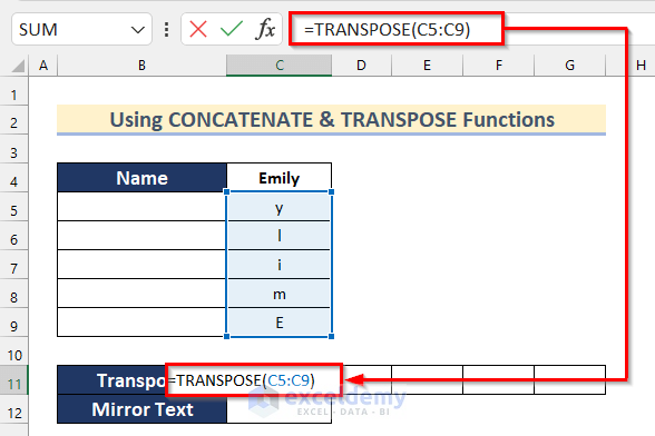
In the TRANSPOSE function, we inserted Cell range C5:C9 as the array.
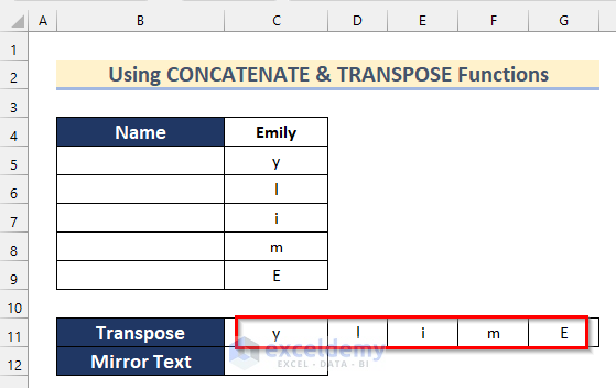
- Get the letters in a modified orientation.
- Select Cell C12.
- Insert the following formula.
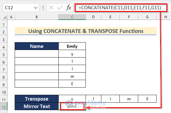
=CONCATENATE(C11,D11,E11,F11,G11)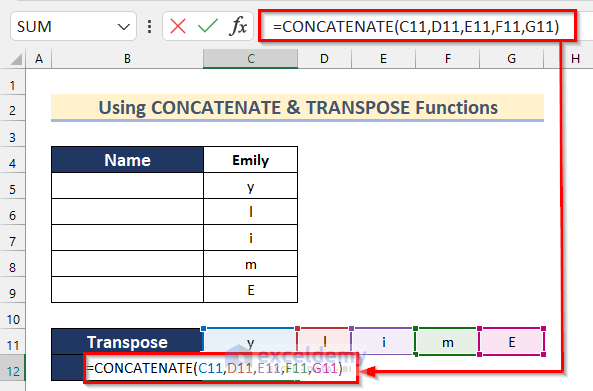
We joined the letters in Cell C11, Cell D1, Cell E1, Cell F1, and Cell G1 using the CONCATENATE function to get the mirror text.
- Get the Mirror Text.
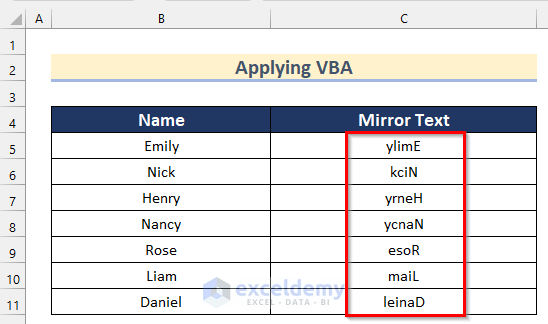
Method 3 – Applying VBA to Mirror Text in Excel
Steps:
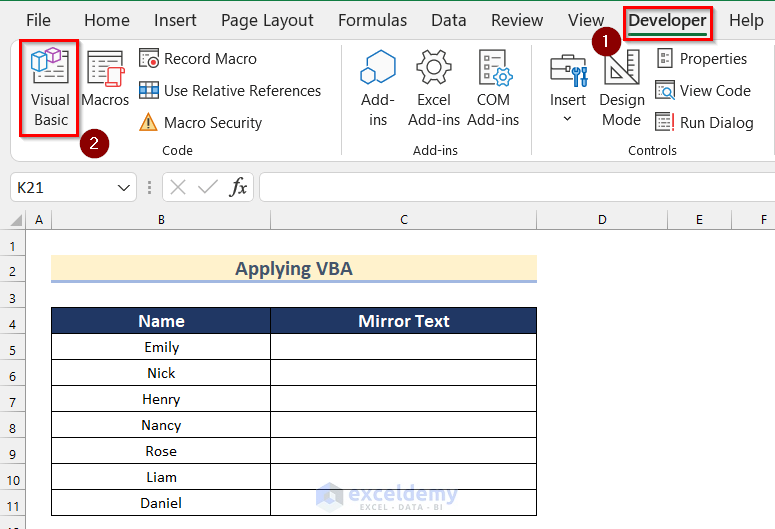
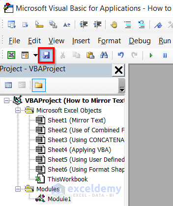
- Go to the Developer tab >> select Visual Basic.
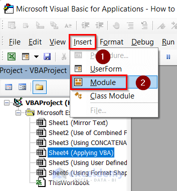
- Write the following code in your Module.
Sub Mirror_Text()
Dim Name As Range
Dim Cell_Value As Range
Set Name = Application.Selection
For Each Cell_Value In Name
    Cell_Value.Offset(0, 1).Value = StrReverse(Cell_Value)
Next Cell_Value
End Sub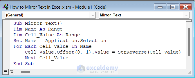
Code Breakdown
- Created a Sub Procedure as Mirror_Text.
- Declared Name and Cell_Value as Range.
- Set the Name range as Application Selection.
- We used a For Each loop for each Cell_Value in Name where we reversed the Cell_Value using StrReverse method and assigned it to the Offset (0,1) Cell.
- Set Cell_Value as Next.
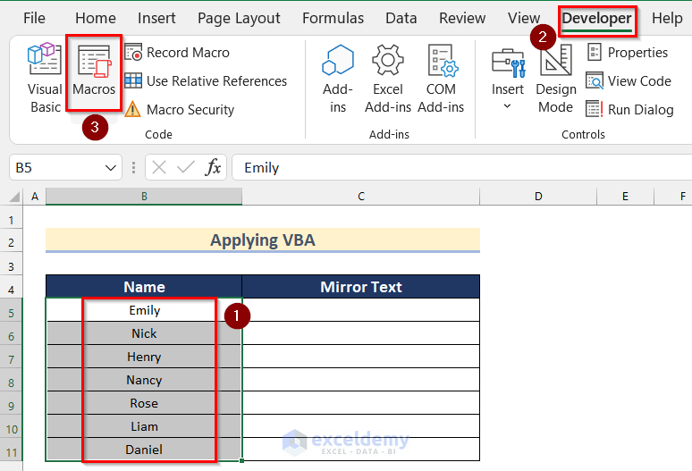
- Select the cell range. I selected the range B5:B11.
- Go to the Developer tab >> click Macros.
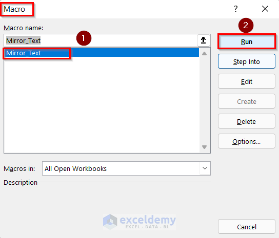
- The Macros box will appear.
- Select Mirror Text.
- Click Run.
- Get all the Mirror Text values.
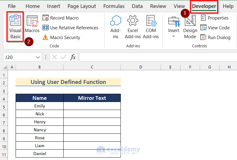
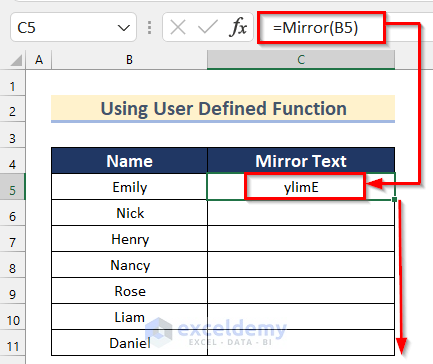
Method 4 – Applying User-Defined Function to Mirror Text in Excel
Steps:
- Go to the Developer tab >> select Visual Basic.
- Insert a module going through the step shown in Method 3.
- Write the following code in your Module.
Function Mirror(Name As String) As String
    Mirror = StrReverse(Trim(Name))
End Function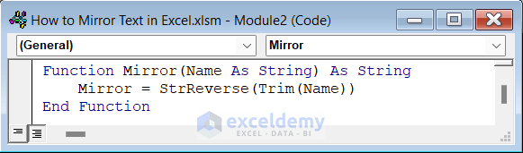
Code Breakdown
- We created a function named Mirror and then used Name as String.
- We used the Trim and StrReverse VBA functions on Name and kept the values in Mirror.
- We ended the function.
- Save the code by following the steps shown in Method 3.
- Select Cell C5.
- Insert the following formula.
=Mirror(B5)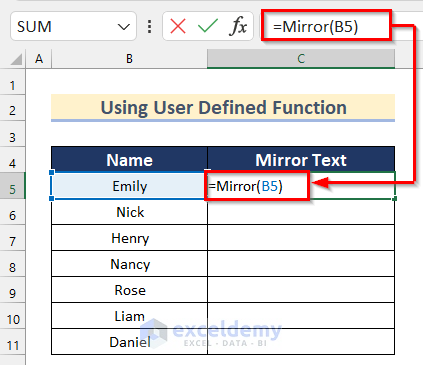
We used the Used Defined function Mirror that we created using VBA and inserted Cell B5 as the input to get Mirror Text.
- Press ENTER to get the Mirror Text.
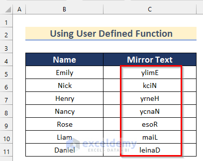
- Drag down the Fill Handle tool to AutoFill the formula for the rest of the cells.
- You will get all the Mirror Text values.
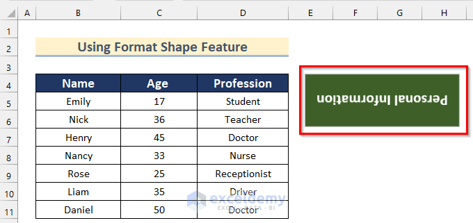
Method 5 – Using Format Shape Feature to Mirror Text in Text Box
Steps:
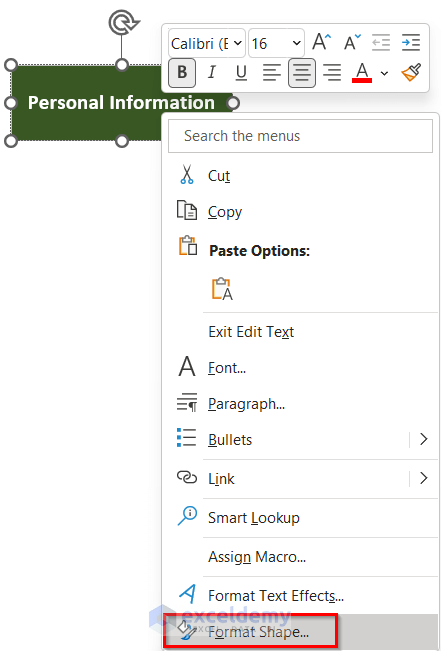
- Select the Text Box and Right-click on it.
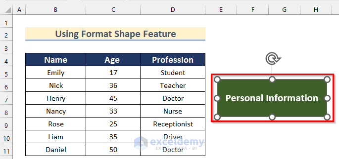
- Select Format Shape.
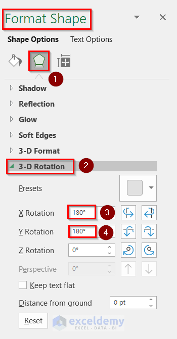
- The Format Shape box will appear.
- Click on the pentagon icon.
- Click on 3-D Rotation.
- Insert 180 as X Rotation and Y Rotation.
- You will get the text in the Text Box in the Mirror version.
Download Practice Workbook
Related Articles
<< Go Back to Text Formatting | Learn Excel
Get FREE Advanced Excel Exercises with Solutions!
