How to Make a Trading Journal in Excel (with Easy Steps)

Last updated: Apr 23, 2024

Let’s say we have a dataset that contains information about several Trades. We will make a trading journal in Excel using Mathematical formulas, the SUM function, and creating a waterfall chart.

Step 1 – Create Dataset with Proper Parameters

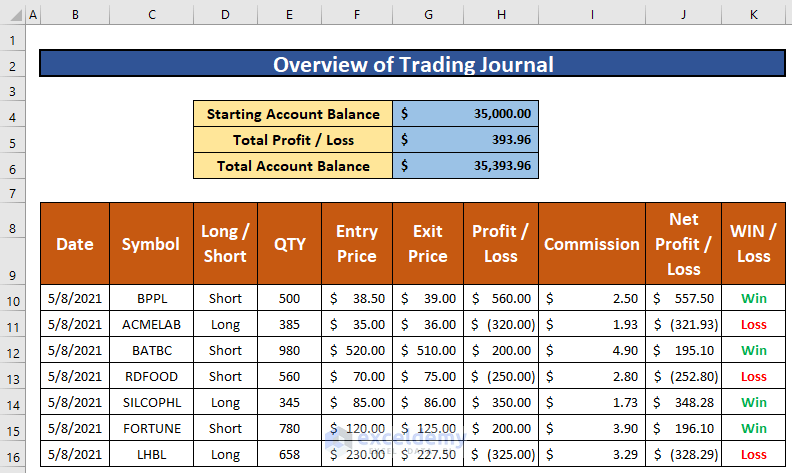
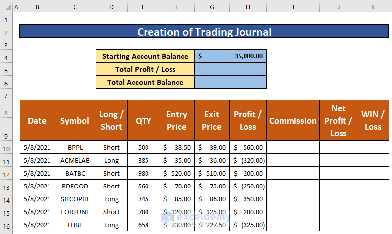
Our dataset contains the trading company name, trade types, the quantity of trades, entry and exit price of trades for a day, profit and loss, commission, and so on.

Create a table and input the information according to the screenshot below.

Step 2 – Calculate Individual Commission and Profit/Loss

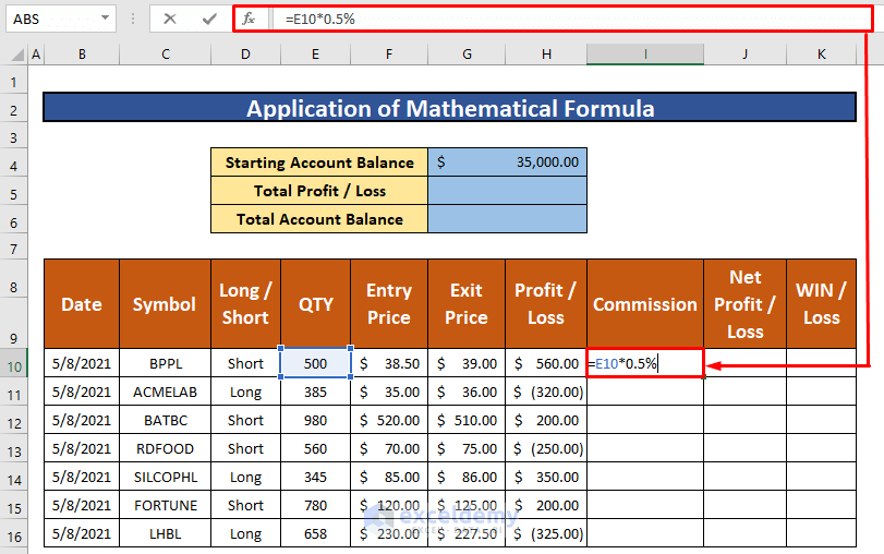
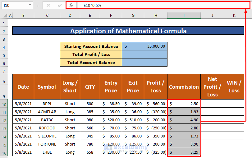
Select cell I10.
Enter the following formula:

=E10*0.5%

E10 is the trade Quantity, and 0.5% is the commission.

Press Enter on your keyboard. You will be able to get the return of the mathematical formula and the return is $2.50.

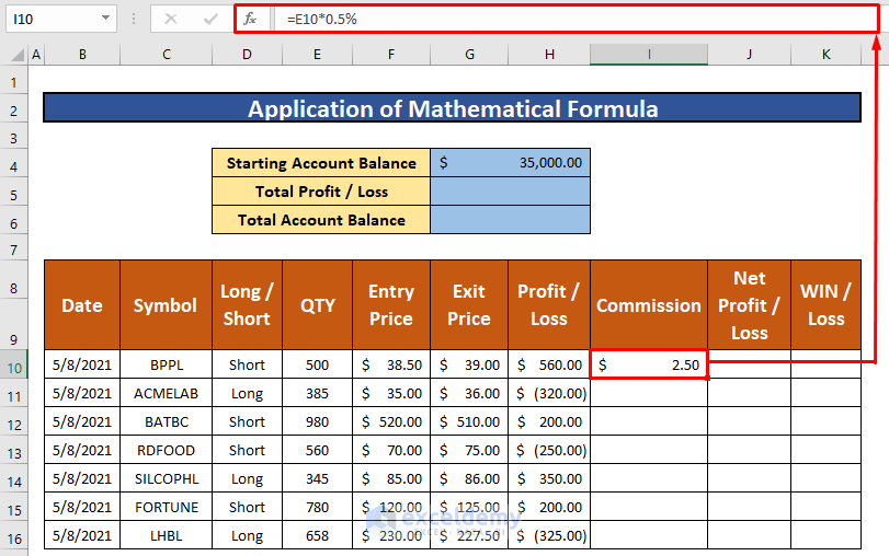
AutoFill the mathematical formula to the rest of the cells in column I.

Select cell J10.
Copy the following formula into it:

=H10-I10

H10 is the Profit or Loss, and I10 is the commission.

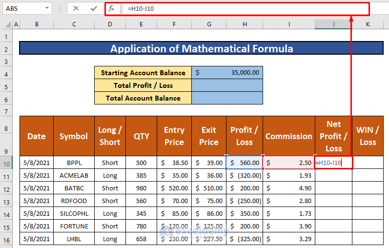
Press Enter.

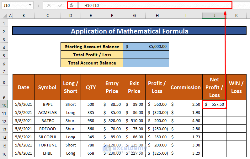
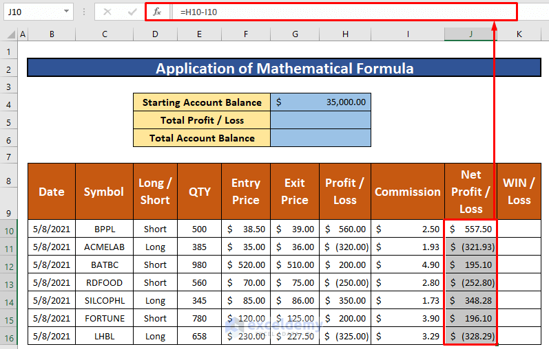
AutoFill the mathematical formula to the rest of the cells in column J.

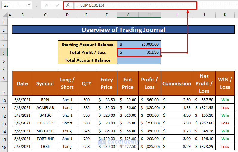
Step 3 – Calculate Total Profit

Input the following formula in H5:

=SUM(J10:J16)

Press Enter.

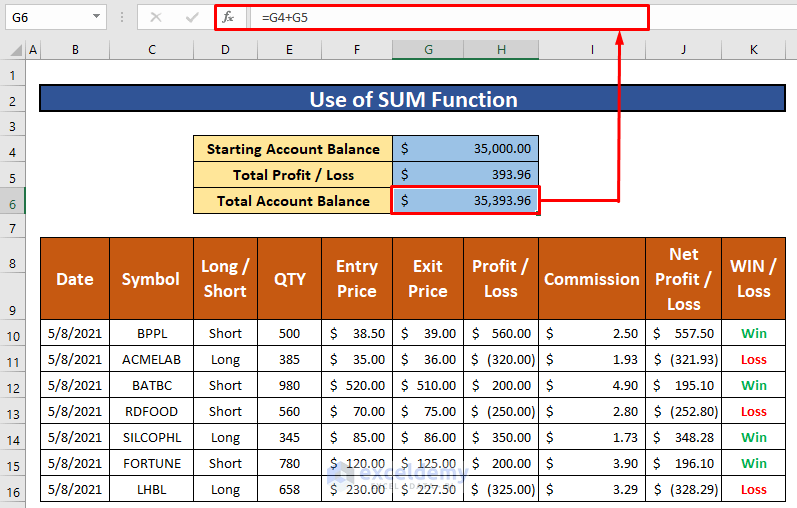
Use the following formula in H6 for the total account balance:

=G4+G5

G4 is the starting account balance, and G5 is the total profit or loss.

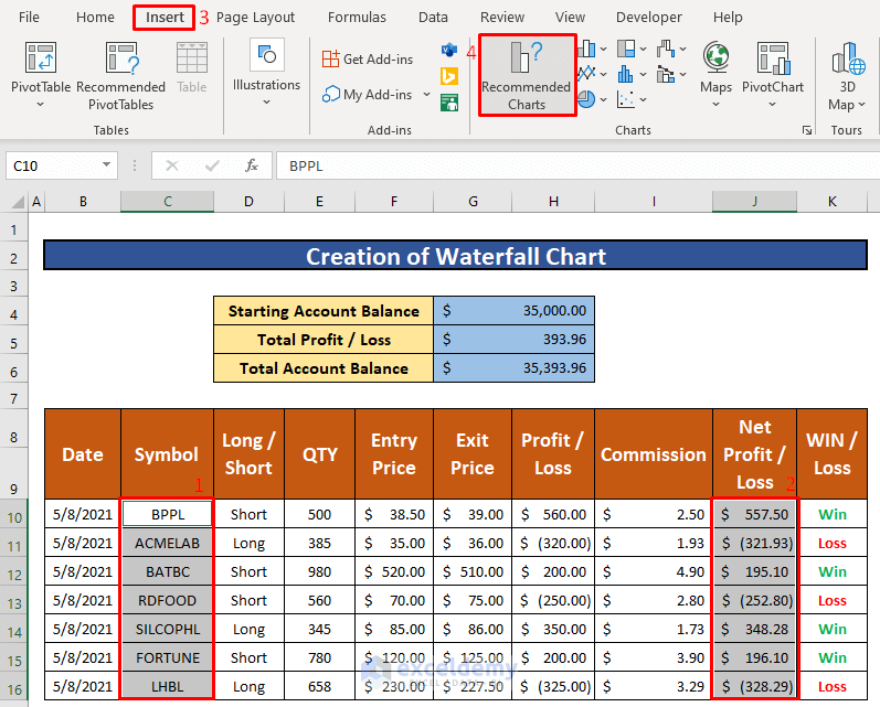
Step 4 – Create Waterfall Chart

Select the range of data to draw a waterfall chart. We selected C10:C16 and J10:J16.
From the Insert tab in the ribbon, go to Recommended Charts

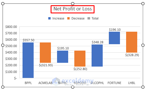
An Insert Chart dialog box will appear in front of you. Go to All Charts and select Waterfall.
Click on OK.

Excel will create a Waterfall chart.

Things to Remember

#N/A! error arises when the formula or a function in the formula fails to find the referenced data.

#DIV/0! error happens when a value is divided by zero(0) or the cell reference is blank.