This is an overview.
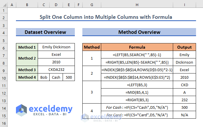
Example 1 – Using the LEFT and the RIGHT Functions to Split One Column into Multiple Columns in Excel
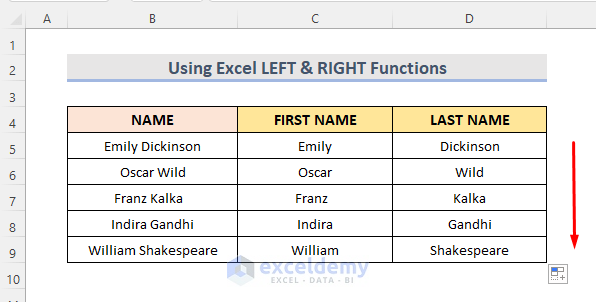
This is the sample dataset. .

Steps:
- Select C5.
- Enter the formula:
=LEFT(B5,SEARCH(" ",B5)-1)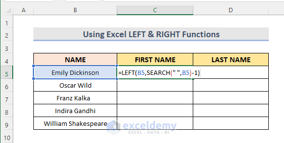
Formula Breakdown
SEARCH(” “,B5)
searches for the space and returns its position.
LEFT(B5,SEARCH(” “,B5)-1)
extracts values to the left.
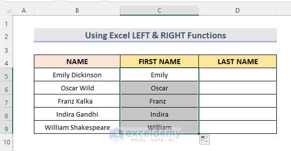
- Press ENTER.
- Drag down the Fill Handle to see the result in the rest of the cells.
- Select D5.
- Enter the formula:
=RIGHT(B5,LEN(B5)-SEARCH(" ",B5))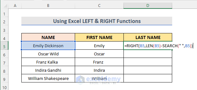
- Press ENTER.
- Drag down the Fill Handle to see the result in the rest of the cells.
Formula Breakdown
SEARCH(” “,B5)
returns the position of the space.
LEN(B5)
returns the total number of characters.
RIGHT(B5,LEN(B5)-SEARCH(” “,B5))
returns the last name.
Read More: How to Split Column by First Space in Excel
Example 2 – Combining the INDEX and the ROW Functions to Split One Column into Multiple Columns in Excel
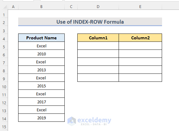
This is the sample dataset.
Steps:
- Select D5.
- Enter the formula:
=INDEX($B$5:$B$14,ROWS(D$5:D5)*2-1)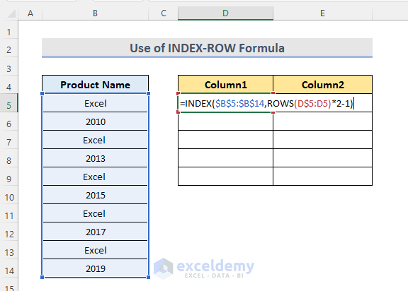
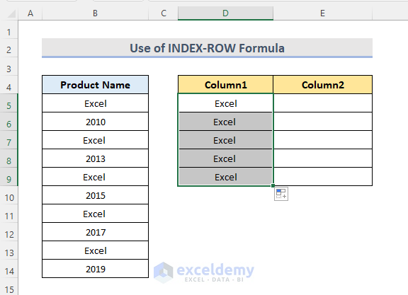
- Press ENTER.
- Drag down the Fill Handle to see the result in the rest of the cells.
Formula Breakdown
ROWS(D$5:D5)*2-1
returns the row number.
INDEX($B$5:$B$14,ROWS(D$5:D5)*2-1)
returns the value in $B$5:$B$14.
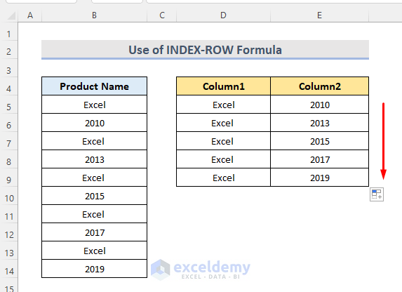
- Select E5.
- Enter the formula:
=INDEX($B$5:$B$14,ROWS(E$5:E5)*2)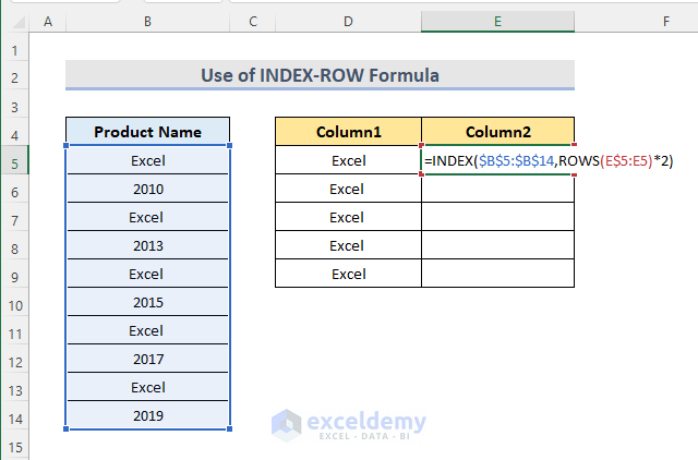
- Press ENTER.
- Drag down the Fill Handle to see the result in the rest of the cells.
Formula Breakdown
ROWS(E$5:E5)*2
returns the row number.
INDEX($B$5:$B$14,ROWS(E$5:E5)*2)
returns the value in $B$5:$B$14.
Read More: Split Date and Time Column in Excel
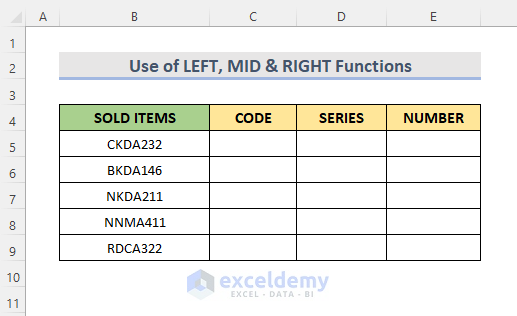
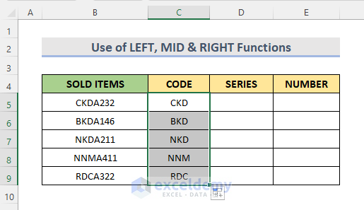
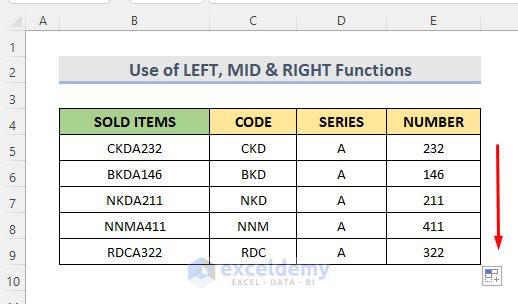
Example 3 – Using the LEFT, MID and RIGHT Functions to Split One Column into Multiple Columns in Excel
In the dataset below, split the sold items column into three columns (CODE, SERIES, NUMBER).
STEPS:
- Select C5.
- Enter the formula:
=LEFT(B5,3)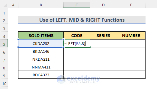
- Press ENTER.
- Drag down the Fill Handle to see the result in the rest of the cells.
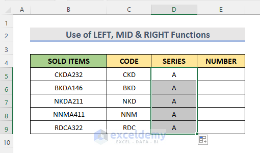
- Select D5.
- Enter the formula:
=MID(B5,4,1)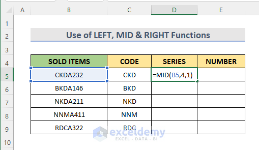
- Press ENTER.
- Drag down the Fill Handle to see the result in the rest of the cells.
- Select E5.
- Use the formula:
=RIGHT(B5,3)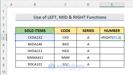
- Press ENTER.
- Drag down the Fill Handle to see the result in the rest of the cells.
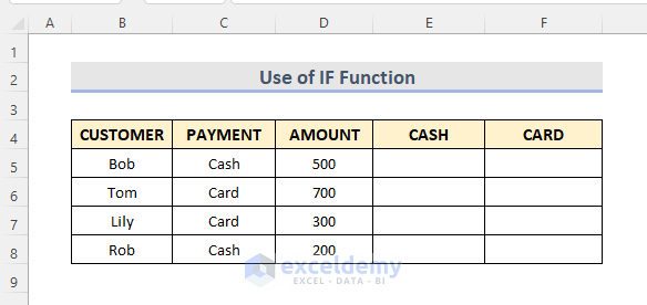
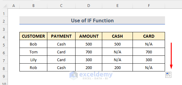
Example 4 – Applying the IF Function to Split a column into Multiple Columns Based on a Value
In the dataset below, split the AMOUNT column into two columns: CASH and CARD.
Steps:
- Select C5.
- Enter the formula:
=IF(C5="Cash",D5,"N/A")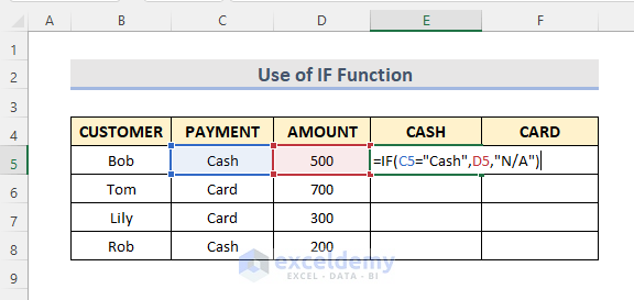
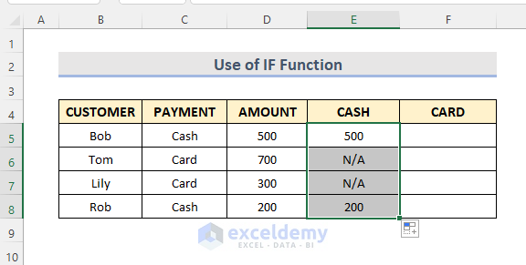
The formula returns the AMOUNT paid Cash in E5. Otherwise, it returns ‘N/A’.
- Press ENTER.
- Drag down the Fill Handle to see the result in the rest of the cells.
- Select F5.
- Enter the formula:
=IF(C5="Card",D5,"N/A")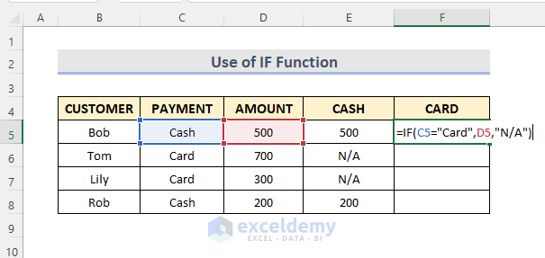
The formula returns the AMOUNT paid by Card in F5. Otherwise, it returns ‘N/A’.
- Press ENTER.
- Drag down the Fill Handle to see the result in the rest of the cells.
Download Practice Workbook
Download the following workbook and exercise.

