What Is the Slope of a Regression Line?
A regression line generally shows the connection between some scatter data points from a dataset. The equation for a regression line is:
y = mx + b
- m = Slope of the Regression Line.
- B = Y-Intercept.
You can also use the following formula to find the slope of a regression line:
m = ∑(x-µx)*(y-µy)/∑(x-µx)²
- µx= Mean of known x values.
- µy= Mean of known y values.
How to Find the Slope of a Regression Line in Excel: 3 Easy Ways
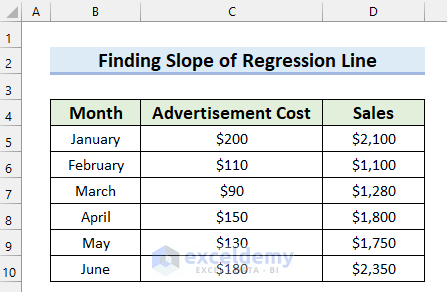
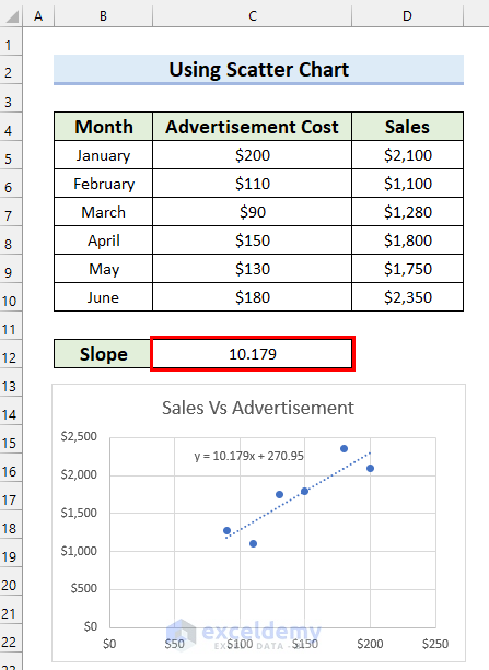
We have the following dataset, containing the Month, Advertisement Cost, and Sales.
Method 1 – Use an Excel Chart to Find the Slope of a Regression Line
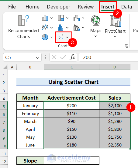
Step 1 – Insert a Scatter Chart
- Select the data range with which you want to make the chart.
- Go to the Insert tab from the Ribbon.
- Select Insert Scatter or Bubble Chart.
- A drop-down menu will appear.
- Select Scatter.
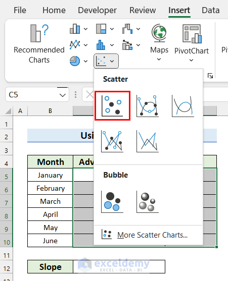
- This inserts a Scatter Chart for your selected data.
- Change the Chart Title.
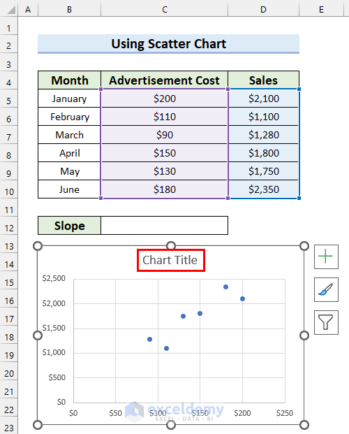
- We have changed the Chart Title.

Step 2 – Add a Trendline
- Select the chart.
- Select Chart Elements.
- Check the Trendline option.
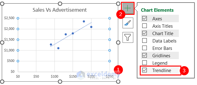
- Here’s the trendline.

Step 3 – Display the Trendline Equation on the Chart and Find the Slope
- Right-click on the Trendline.
- Select Format Trendline.
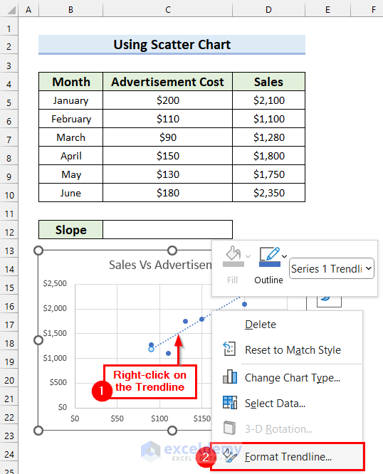
- The Format Trendline task pane will appear on the right side of the screen.
- Select the Trendline Options tab.
- Check the Display Equation on chart option.
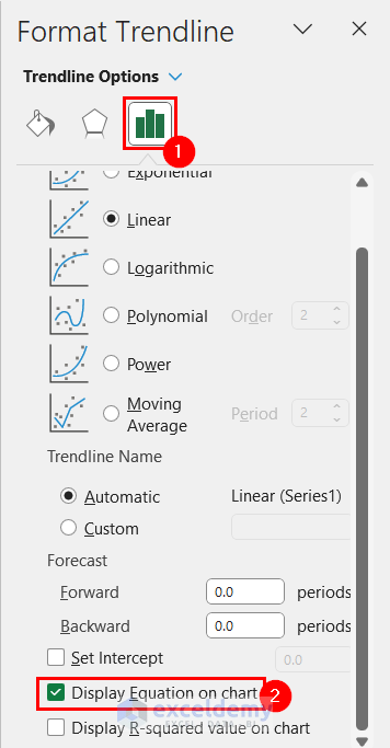
- You will be able to see the equation for the Trendline on the chart.
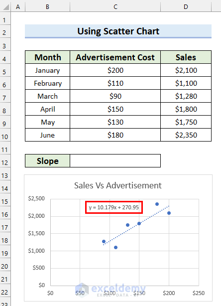
- Determine the Slope from the equation (the part before the x) and write it down in your preferred location.
Read More: How to Find Instantaneous Slope on Excel
Method 2 – Apply the SLOPE Function to Calculate the Slope of a Regression Line in Excel
Steps:
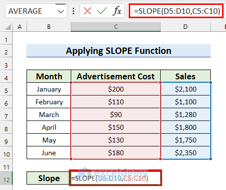
- Select the cell where you want the Slope. We selected Cell C12.
- Insert the following formula.
=SLOPE(D5:D10,C5:C10)
- Press Enter to get the result.
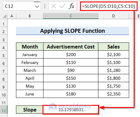
In the SLOPE function, we selected cell range D5:D10 as known_ys, and C5:C10 as known_xs. The formula will return the slope of the regression line for these data points.
Read More: How to Find the Slope of a Line in Excel
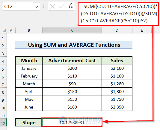
Method 3 – Determine the Slope of a Regression Line Manually Using SUM and AVERAGE Functions
Steps:
- Select the cell where you want the Slope.
- Insert the following formula in the selected cell:
=SUM((C5:C10-AVERAGE(C5:C10))*(D5:D10-AVERAGE(D5:D10)))/SUM((C5:C10-AVERAGE(C5:C10))^2)
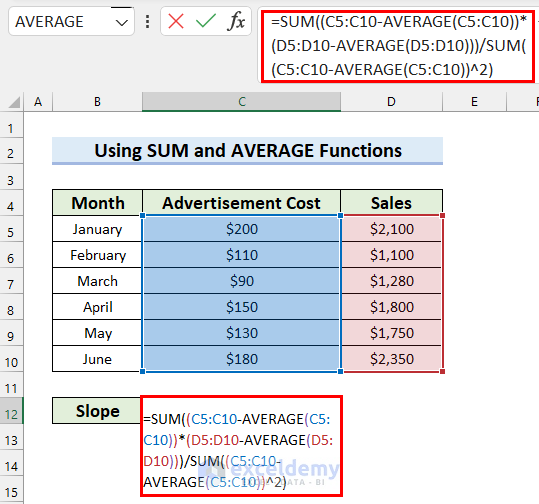
- Press Enter to get the result.
How Does the Formula Work?
- AVERAGE(C5:C10): The AVERAGE function returns the average of cell range C5:C10.
- (C5:C10-AVERAGE(C5:C10)): The average is subtracted from the cell range C5:C10.
- AVERAGE(D5:D10): The AVERAGE function returns the average of cell range D5:D10.
- (D5:D10-AVERAGE(D5:D10): The average is subtracted from the cell range D5:D10.
- (C5:C10-AVERAGE(C5:C10))*(D5:D10-AVERAGE(D5:D10)): The formula multiplies the results it got from the previous formulas.
- SUM((C5:C10-AVERAGE(C5:C10))*(D5:D10-AVERAGE(D5:D10))): The SUM function returns the summation of these values.
- (C5:C10-AVERAGE(C5:C10))^2: The average of cell range C5:C10 is subtracted from cell range C5:C10. And then raised to the power of 2.
- SUM((C5:C10-AVERAGE(C5:C10))^2): The SUM function returns the summation of the values it got from the previous calculation.
- SUM((C5:C10-AVERAGE(C5:C10))*(D5:D10-AVERAGE(D5:D10)))/SUM((C5:C10-AVERAGE(C5:C10))^2): The first summation is divided by the second summation.
Read More: How to Find Slope of Logarithmic Graph in Excel
Practice Section
We have provided a practice sheet for you to practice how to find the slope of a regression line in Excel.

Download the Practice Workbook
Related Articles
<< Go Back to Excel SLOPE Function | Excel Functions | Learn Excel
Get FREE Advanced Excel Exercises with Solutions!
