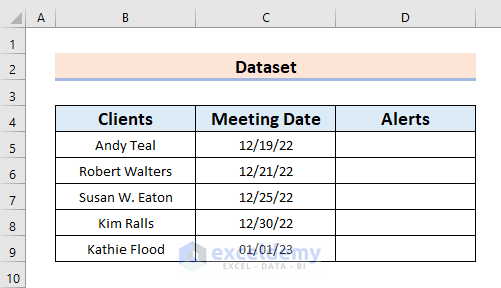
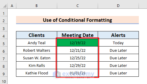
In the below dataset we have three columns displaying Client names, Meeting Dates, and Alerts.
Method 1 – Using the IF Function to Create Alerts Automatically
Steps:
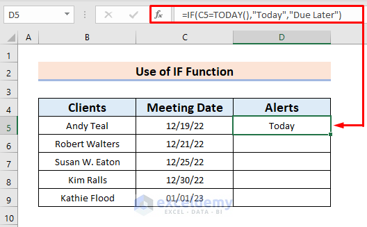
- Enter the following formula in cell D5:
=IF(C5=TODAY(),"Today","Due Later")- Press Enter to see the result in D5. The return is TODAY.
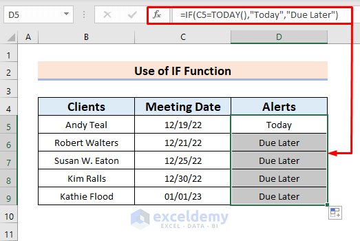
- Use the Fill Handle tool to AutoFill the rest of the cells in column D.
Formula Breakdown
- TODAY() returns the current day in a date format.
- =IF(C5=TODAY(),”Today”,”Due Later”) verifies whether the conditions are TRUE or FALSE. If TRUE, then it returns Today, and if FALSE, it thoroughly returns Due Later.
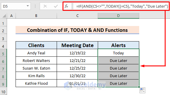
Method 2 – Combining IF, TODAY & AND Functions to Show Alerts
Steps:
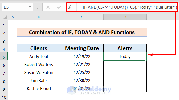
- Enter the following formula in cell D5:
=IF(AND(C5<>"",TODAY()=C5),"Today","Due Later")
- Press Enter.
- AutoFill the range by dragging the formula cell down.
- The alerts pop up in the dataset.
Formula Breakdown
- TODAY() returns the current day in a date format.
- AND(C5<>””,TODAY()=C5) checks whether the statement is TRUE and returns only the TRUE
- =IF(AND(C5<>””,TODAY()=C5),”Today”,”Due Later”) verifies whether the conditions are TRUE or FALSE. If TRUE then it returns Today and if FALSE, it thoroughly returns Due Later.
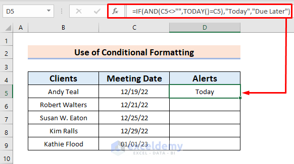
Method 3 – Using the Conditional Formatting Feature to Display Alerts Notifications
Steps:
- Enter the following formula in D5:
=IF(AND(C5<>"",TODAY()=C5),"Today","Due Later")- Press Enter to get the result.
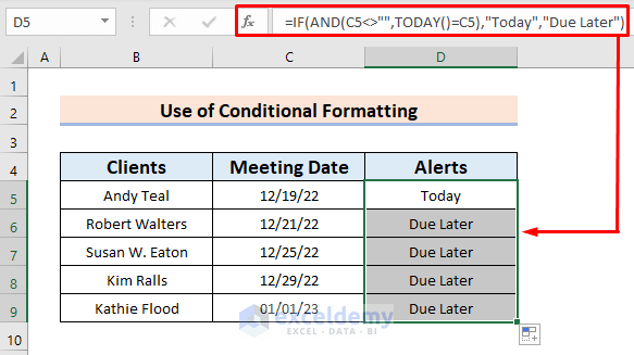
- Drag the AutoFill Handle up to cell D9.
- The alert texts are in the range.
- Select the range C5:C9.
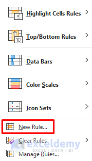
- Go to the Home tab and click the Conditional Formatting option.
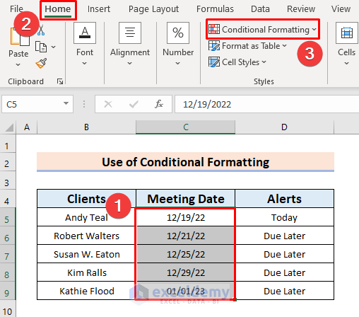
- A drop-down box appears.
- Tap the New Rule option.
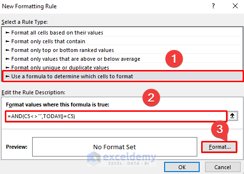
- The New Formatting Rule pops up.
- Choose the option Use a formula to determine which cells to format.
- In the Edit the Rule Description box, type = and paste the formula.
- hit Format.
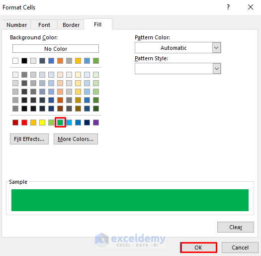
- The Format Cells menu option opens.
- To illustrate, we selected Green and pressed OK.
- Our meeting date is highlighted.
Method 4 – Running an Excel VBA Code to Get Pop-up Alerts
Steps:
- Go to the Developer tab and click Visual Basic.
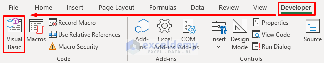
- The Visual Basic window pops up.
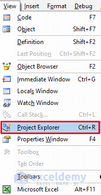
- Click View > Project Explorer > This Workbook to open a workbook.
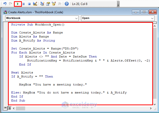
- Enter the VBA code below:
Private Sub Workbook_Open()
Dim Create_Alerts As Range
Dim Alerts As Range
Dim A_Notify As String
Set Create_Alerts = Range("D5:D9")
For Each Alerts In Create_Alerts
    If Alerts <> "" And Date = DateDue Then
        A_Notify = A_Notify & " " & Alerts.Offset(0, -2)
    End If
Next Alerts
If A_Notify = "" Then
    MsgBox "You have a meeting today."
Else: MsgBox "You do not have a meeting today." & A_Notify
End If
End Sub
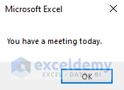
- Press the green Run button.
- We get the desired pop-up alert message.
Download the Practice Workbook
Download this workbook to practice.
Related Articles
- How to Generate Automatic Email Alerts in Excel
- How to Disable Alerts in Excel VBA
- How to Set Due Date Reminder Formula in Excel
- How to Set Due Date Reminder in Excel
<< Go Back to Alerts in Excel | Learn Excel
Get FREE Advanced Excel Exercises with Solutions!
