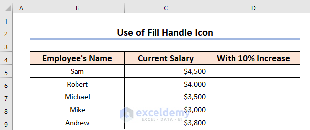
How to Copy a Formula in Excel with Changing Cell References (14 Methods)

Method 1 – Dragging Fill Handle Icon

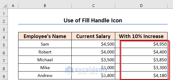
Suppose a company has decided to increase the salary of five specific employees by 10%. You have a chart with employees’ names and their current salaries. To find their new salaries after the increase, multiply each employee’s current salary by 1.1 (which represents a 10% increase).

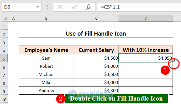
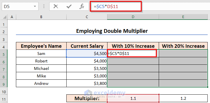
Select cell D5.
Type =. then select cell C5 and multiply it by 1.1.

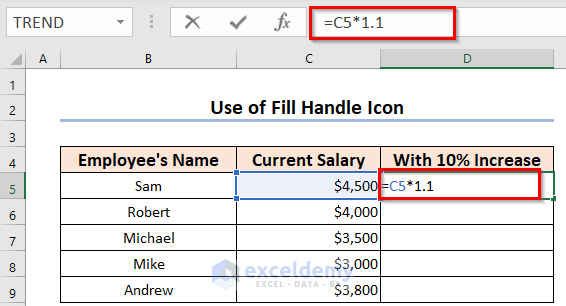
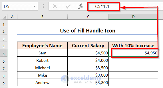
Press ENTER to see Sam’s new salary in cell D5.

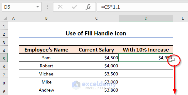
To calculate new salaries for all other employees, use the Fill Handle icon: Click and drag from the bottom right corner of cell D5 down to cell D9.

Method 2 – Double Clicking Fill Handle

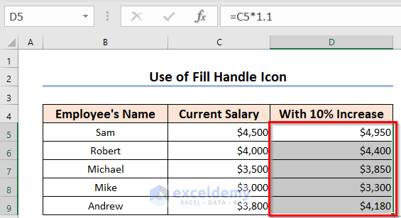
Alternatively, double-click the Fill Handle icon (‘+’ sign) after calculating the first cell (D5).

This action will apply the formula to all employees’ salaries at once.

Read More: How to Copy SUM Formula in Excel

Method 3 – Creating an Excel Table

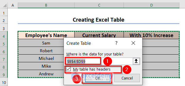
Select the entire section.
Go to the Insert tab and choose the Table option.

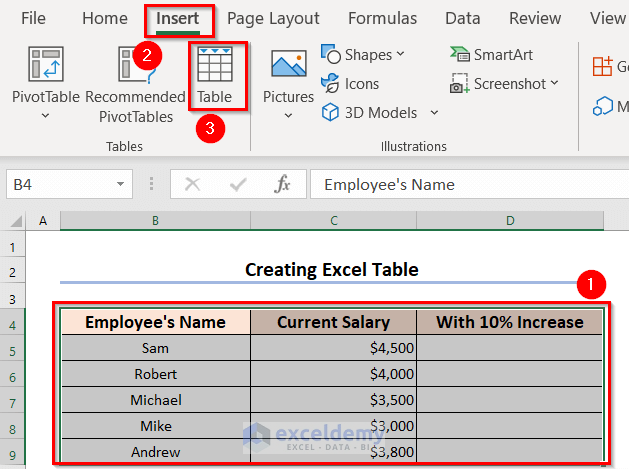
In the Create Table dialog box, ensure My table has headers is checked.
Press OK.

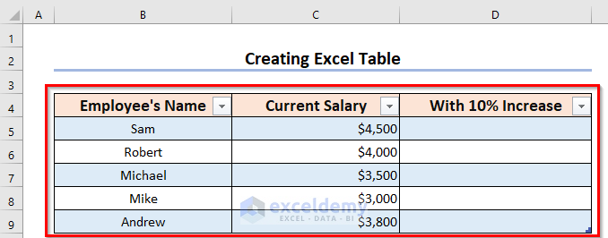
At this time, the table will appear with headers.

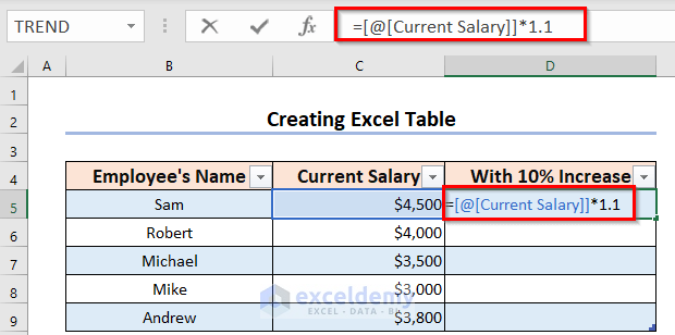
In cell D5, enter =C5*1.1 and press ENTER.

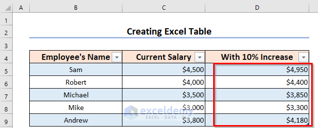
You will get the results as follows:

Method 4 – Copying Formula to Non-Adjacent Cells

When dealing with gaps between rows or columns, copying the formula manually is necessary.

Right-click cell D5.

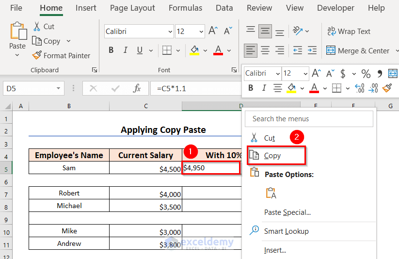
Hold CTRL and select cells D7, D8, D10, and D11.

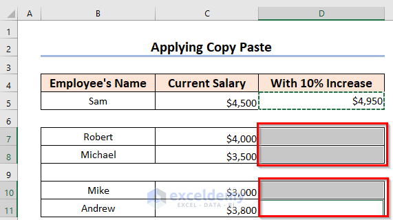
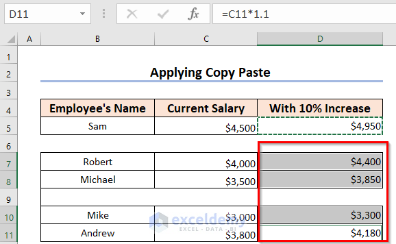
Right-click again and choose Paste Options to get the desired results.

Method 5 – Using Single Formula for Multiple Columns

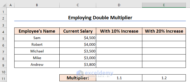
To calculate salaries with different multipliers (e.g., 10% and 20%), select the array D5:E9.

(Here, if you are using an older version of Excel than 2013 then press F2 to enable editing at D5. Furthermore, we used the Microsoft 365 version here.)

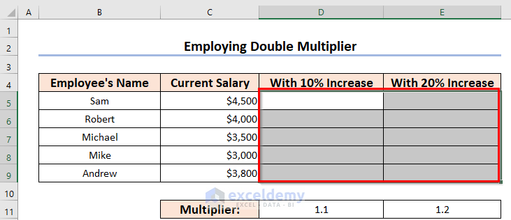
Enter the formula to multiply cell C5 by D11 (1st multiplier), ensuring proper mixed cell references.

Press the CTRL+ENTER keys and you’ll see the 10% and 20% increased salaries for all employees.

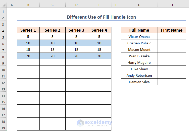
Method 6 – Using Fill Handle Icon Differently

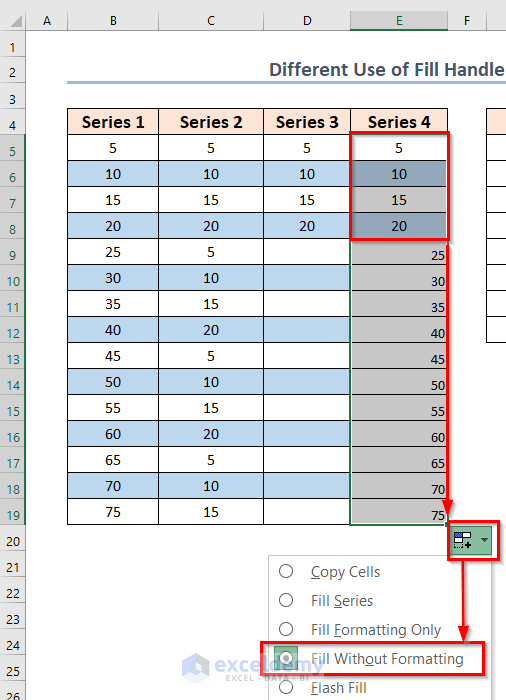
Let’s explore a series of multipliers (in this case, multiples of 5). How can you quickly generate all the subsequent values in a column with just one action?

Select cells from B5 to B8.

Hover your mouse over the bottom-right corner of cell B8 (where you’ll find the Fill Handle icon).
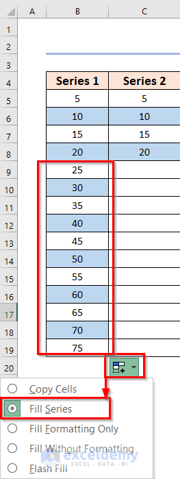
Drag the Fill Handle down to fill the series.

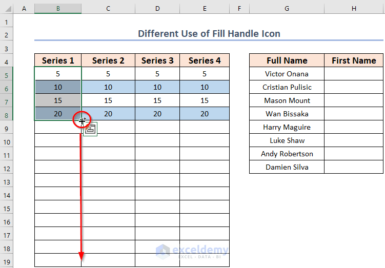
As a result, you’ll obtain the desired values for the multipliers of 5. Excel automatically recognizes this as a Fill Series operation.

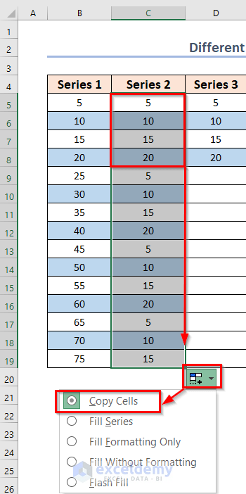
Other Copy Options:

Copy Cells: This option repeats the first four selected cells downward.
- If you choose Copy Cells, the 1st 4 cells you’ve selected before will be copied downward again and again.

Fill Formatting Only: Copies only the cell formatting (background, borders, etc.), not the values.

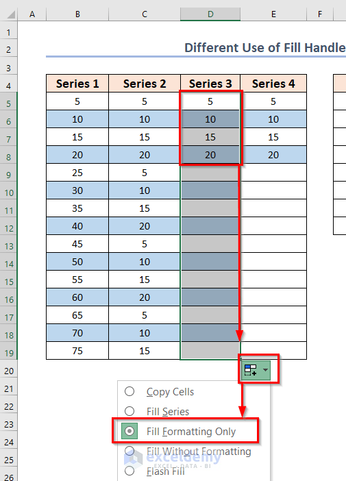
Fill Without Formatting: Provides the entire series without copying cell background patterns.

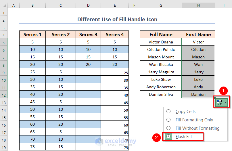
Interesting Scenario: Extracting First Names Suppose you have a list of full names, and you want to extract only the first names. Follow these steps:

In a First Name column, enter the first name for the initial entry.
Drag the Fill Handle icon down to cover the remaining cells.

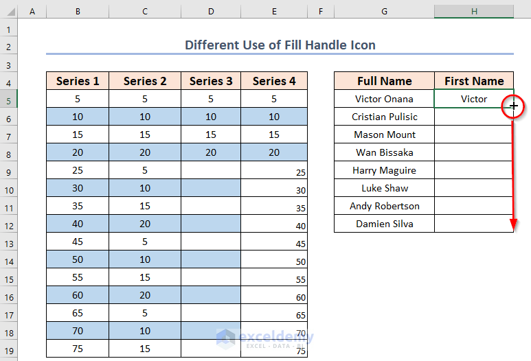
Select Flash Fill.

All the first names will populate automatically in the column.

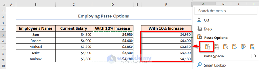
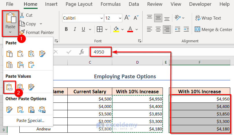
Method 7 – Applying Different Paste Options

Similar to copy options, paste options offer various choices.

Let’s say you want to copy data from column D to F, including formulas.

Remember to lock column C to avoid errors during pasting.

Right-click cell F5 to explore different paste options:

- Formulas: Includes the formulas used in column D.

- Values (123): Copies only the values, excluding formulas.

- Paste Link: Displays calculated values in column F, linking to the functions assigned in column D.

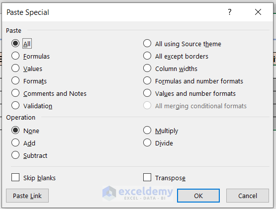
There are other Paste options that you can find through Paste Special tab.

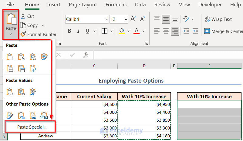
You can select a wide variety of options to paste the values or formulas or both depending upon your required criteria.

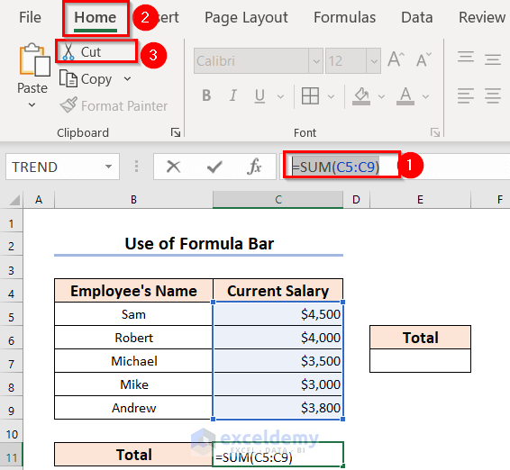
Method 8 – Copying Function(s) from Formula Bar

Calculate the total current salaries of the five employees using the SUM function.

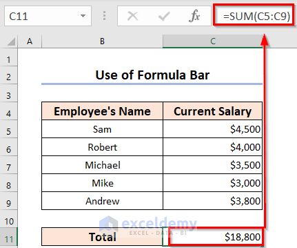
Focus on the Formula Bar and cut the formula (instead of copying). Cutting ensures proper cell references.

Paste the formula into cell E7.

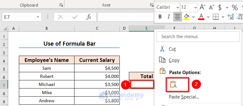
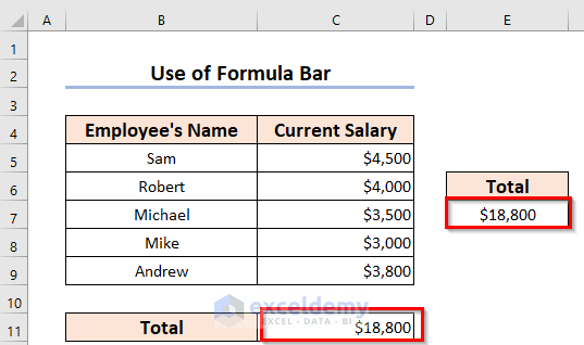
The calculated value will appear.

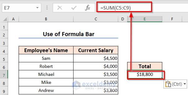
Note: That cutting the formula removes the value from cell C11, so you’ll need to paste the function there again to restore it.

Method 9 – Preventing Changes to Cell References

In this method, we’ll address the challenge of maintaining consistent cell references. Suppose you want to calculate increased salaries for employees with both 10% and 20% increments.

Select the array D5:E9.
In cell D5, multiply C5 by D11 (representing a 10% increase).

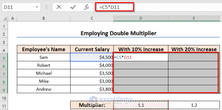
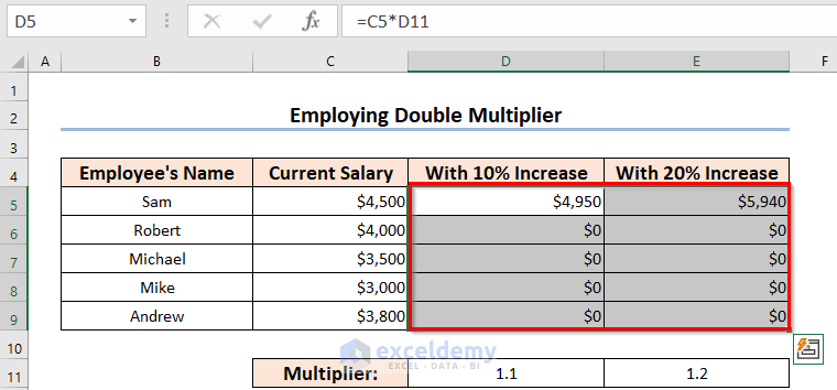
Press CTRL+ENTER.
You’ll notice that only Sam’s salary has been calculated, while the others remain unchanged. The reason is that cell references are not locked.

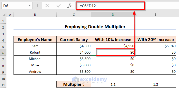
Let’s view cell D6. Look at the Formula Bar and you’ll see the calculation has been executed based on the multiplication between Robert’s current salary(C6) and an empty cell (D12)!

Basically, this is why the result has been displayed as $0.

To lock the references:

In the Formula Bar, add a $ sign before C (to lock column C).
Add another $ sign before 11 (to lock row 11, which contains the multipliers).
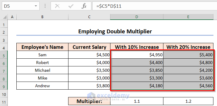
Press CTRL+ENTER to obtain the expected calculations:

Under column D, all employees’ salaries will be multiplied by 1.1 (from D11).
Under column E, salaries with 20% increments will be calculated using the multiplier 1.2 (from E11).

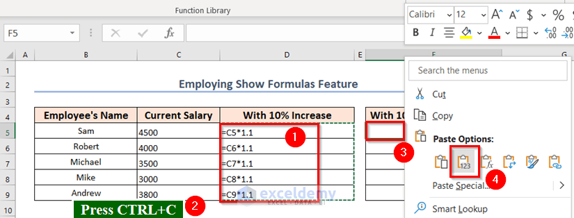
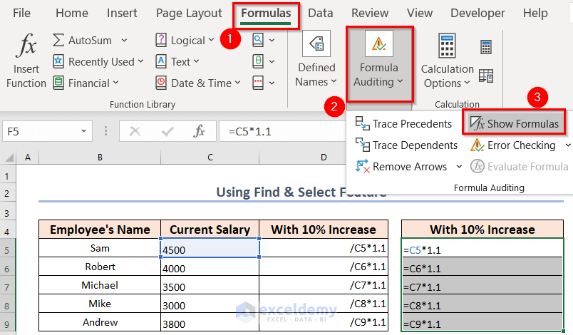
Method 10 – Using Show Formulas Feature

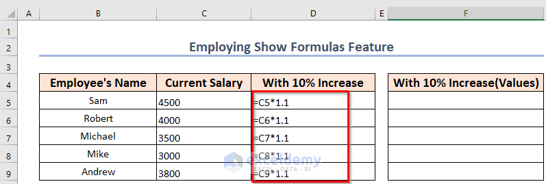
Calculate the increased salaries as before.
Under the Formulas tab, click Show Formulas.

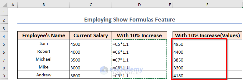
In column D, you’ll see the executed functions in each cell.

Copy these formulas using CTRL+C.
Create a new chart under column F.
Paste the formulas at F5 using the Values(V) option.

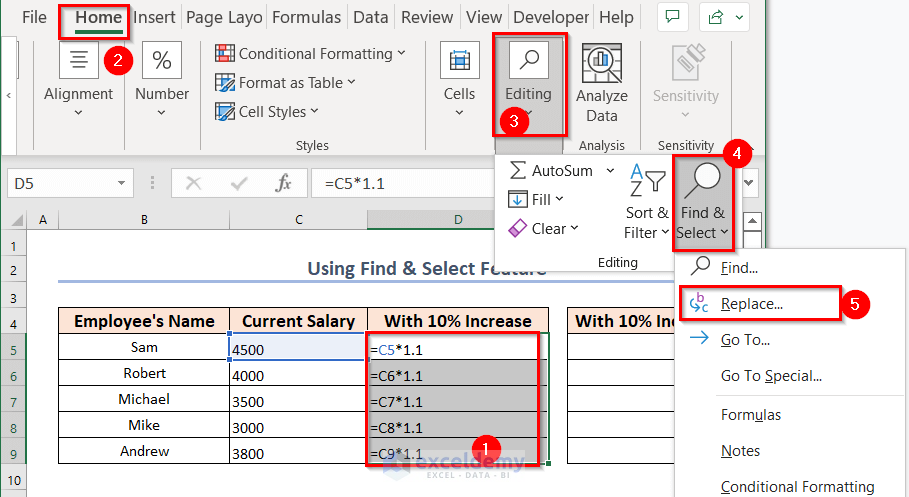
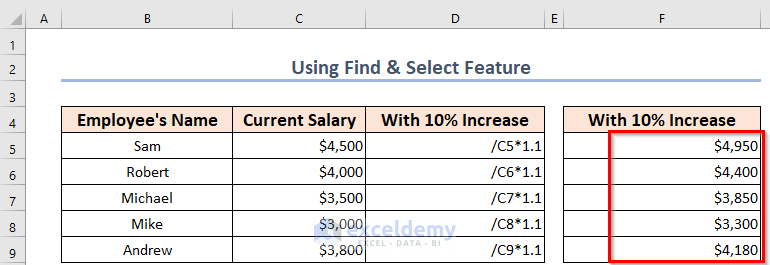
Method 11 – Applying ‘Find & Replace’

Select the column range D5:D9.
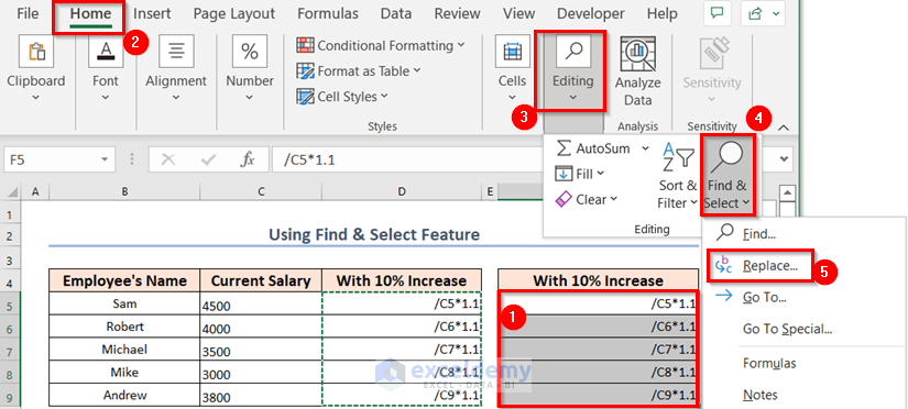
Go to the Home tab and choose Replace from the Editing menu.
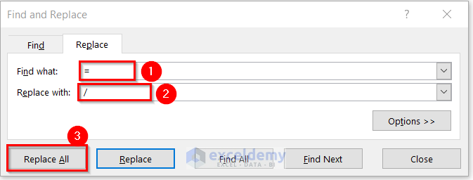
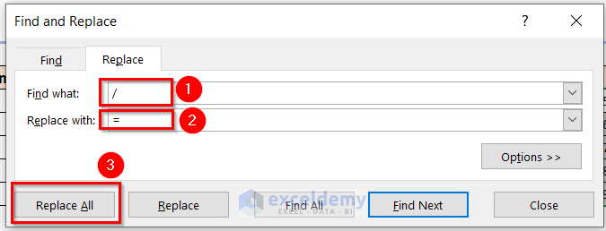
In the Find and Replace dialog box:

- Replace the ‘=’ symbol with ‘/’ or any other symbol which has not been used already in the spreadsheet.
- Click Replace All.

Confirm in the Microsoft Excel box.

Close the Find and Replace dialog.
Column D now contains text strings (not formulas).
Paste column D into column F.
Open the Find & Replace tab again.

Reverse the symbols used earlier.
Choose Replace All to convert text strings back to number functions.

Press OK.

Turn off Show Formulas to see the calculated values in column F.

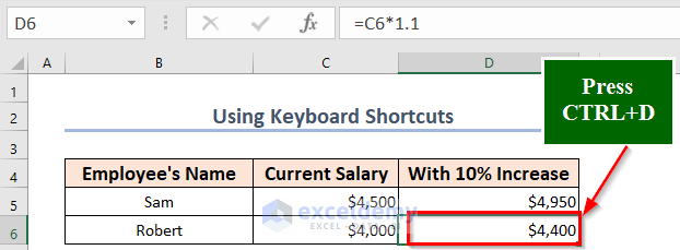
Method 12 – Using CTRL+D & CTRL+R for Immediate Next Cell to Fill

You can use keyboard shortcuts like CTRL+D or CTRL+R to fill cells sequentially. Here’s how:

After calculating the initial value in cell D5, move to cell D6.
Use CTRL+D to fill downward (copy the formula).

Similarly, go to cell D8 and press CTRL+R to fill to the right.

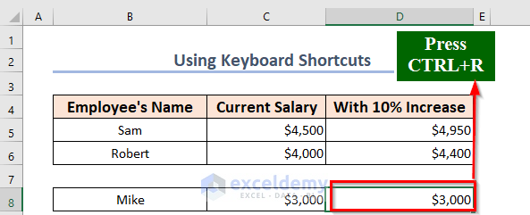
This method is useful for small data sets.

Method 13 – Creating a Notepad and Pasting Formulas

Expose the formulas in column D (using the Show Formulas feature).
Copy the formulas from column D to a Notepad.

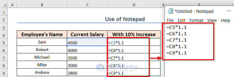
Paste the formulas from the Notepad into column F.

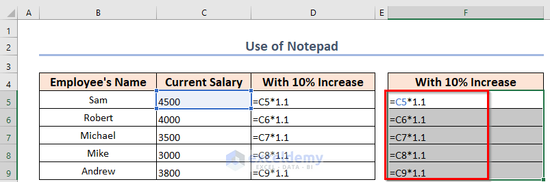
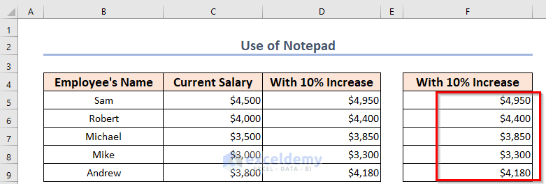
Turn off the Show Formulas view to display the calculated values.

This method helps track data while keeping formulas hidden during copying.

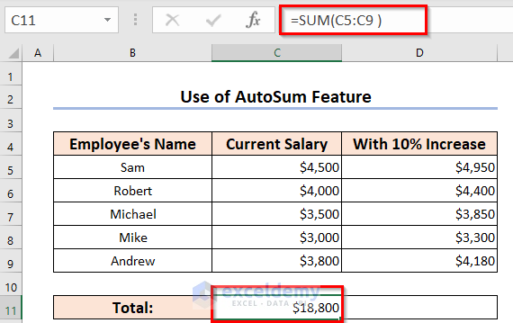
Method 14 – Using AutoSum or SUBTOTAL Function

AutoSum:
- Under the Home tab, choose AutoSum to access basic functions (e.g., SUM, average, count).

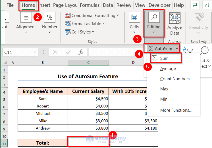
Select a cell and click Sum to calculate the sum of a range (e.g., Column C).

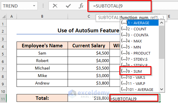
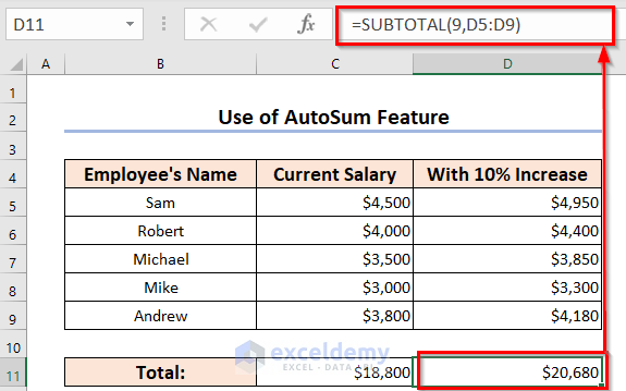
SUBTOTAL Function:
- Similar to AutoSum, SUBTOTAL offers various functions (e.g., SUM, COUNT) with additional options.
- Use parameter 9 for SUM.

Here we also did the summation for Column C with the help of the SUBTOTAL function.