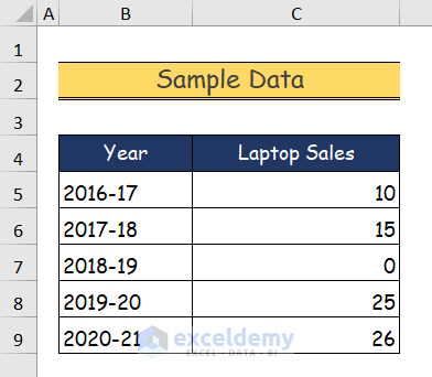
Zero values often create difficulties while visualizing data in a chart. Here are 5 effective methods to hide these values from Excel charts. We will use the sample dataset below to illustrate the methods.
Method 1 – Using the Filter Command to Hide Zero Values in an Excel Chart
Steps:
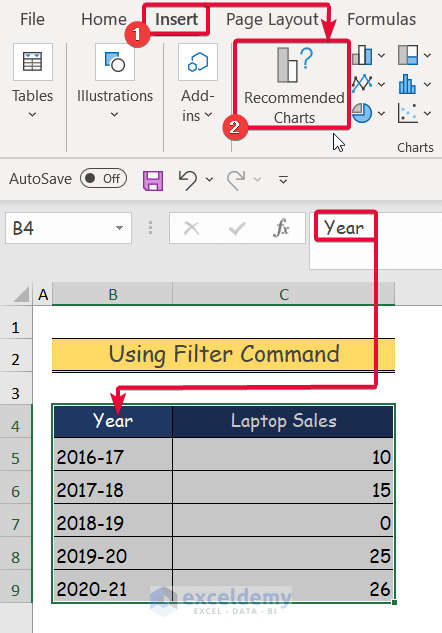
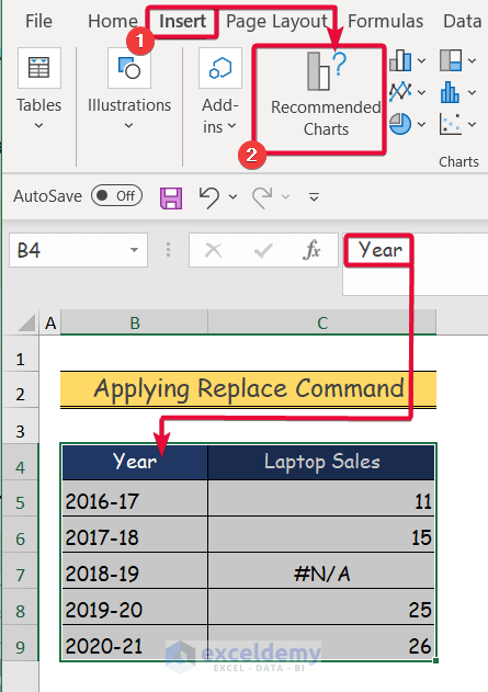
- Select the entire dataset. We will select the cells in the range B4:C9.
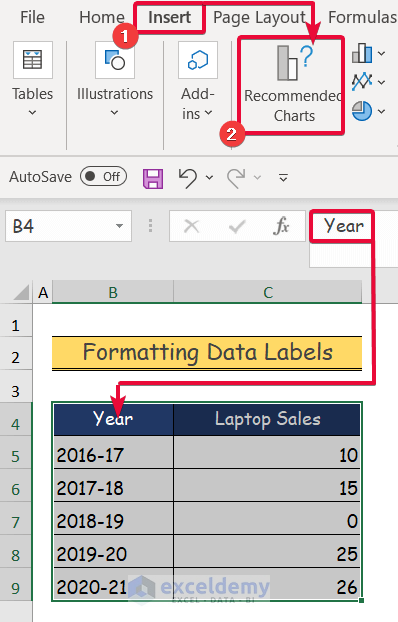
- Go to the Insert tab.
- From the Chart group, select Recommended Charts.
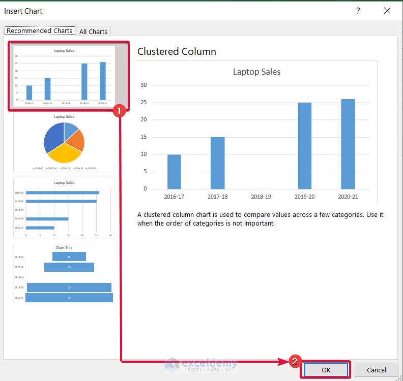
- Select any chart of your preference. We will select the Clustered Column chart.
- Click OK.
- The chart will be added to the dataset.

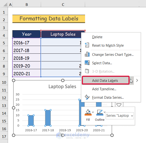
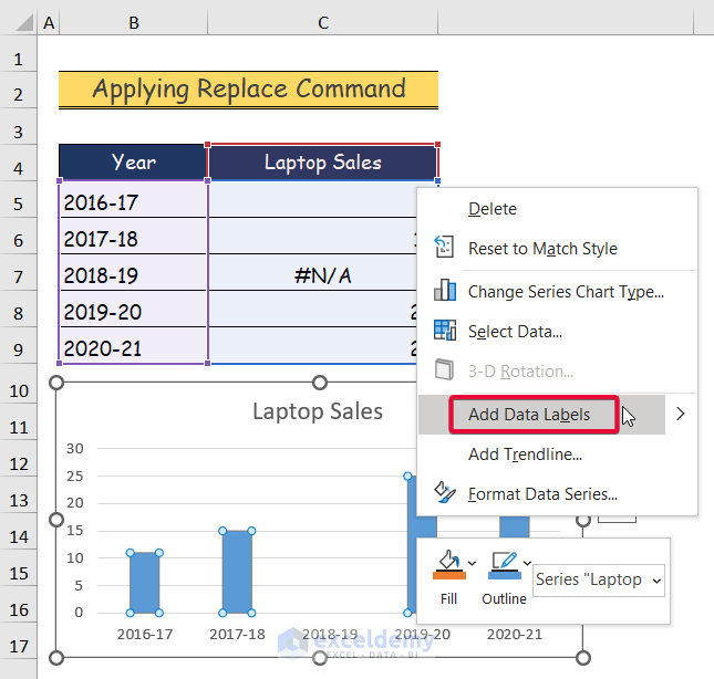
- Right-click on the chart.
- From the available options, select Add Data Labels.
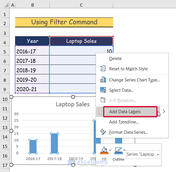
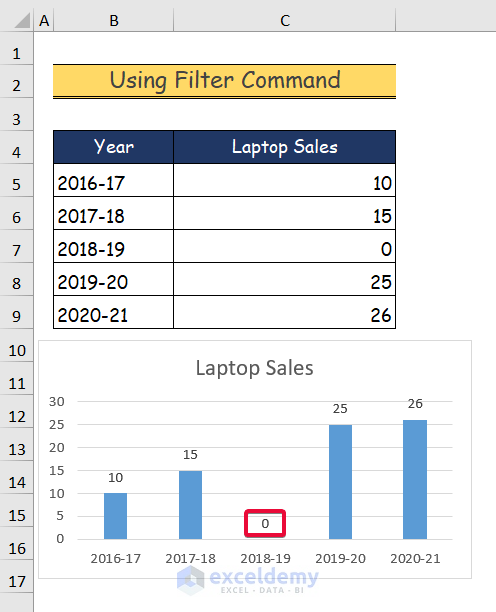
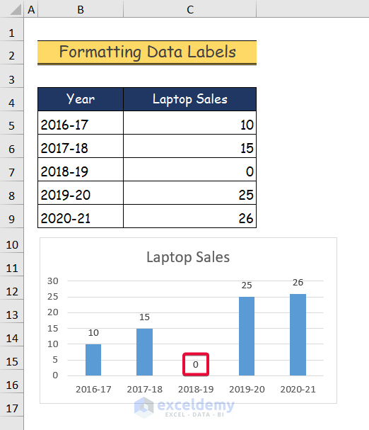
- You will find that a zero value is present in your chart.
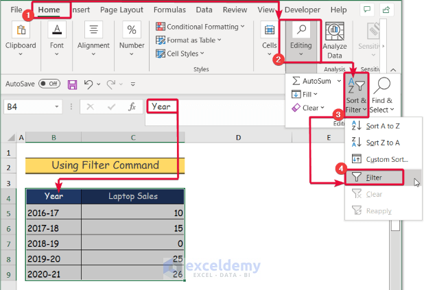
- Go to the Home tab.
- Navigate to the Editing group.
- Select Sort & Filter.
- From the drop-down options, select the Filter command.
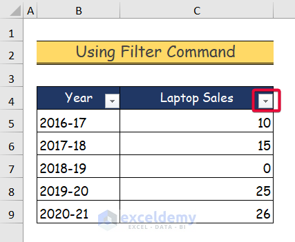
- A filter option will be added to the header rows.
- Select the filter option of the header row that contains the zero value.
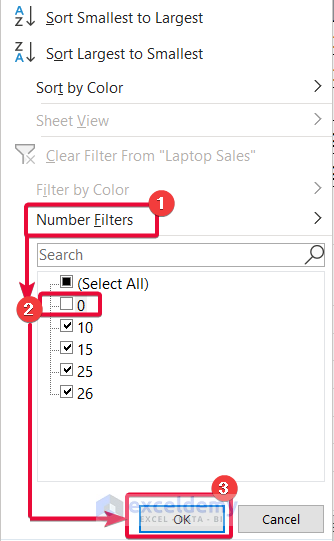
- From the filter dialogue box, go to the Number filters.
- Uncheck the box beside the Zero option.
- Select OK.
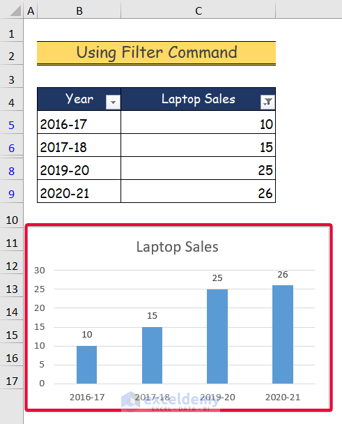
- Our chart is free of zero values.
Method 2 – Formatting Data Labels to Hide Zero Values in an Excel Chart
Steps:
- Select the entire dataset. The selected data is in the cell range of B4:C9.
- Go to the Insert tab.
- Select the Recommended Charts tab in the Chart group.
- Select any chart that suits your needs. We will go with the Clustered Column chart.
- Click OK.
- The chart will be included in our dataset.
- Right-click the chart.
- Choose Add Data Labels from the list of options.
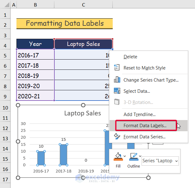
- There’s a zero value in our chart.
- Right-click the zero value.
- Select Format Data Labels from the available options.
- The Format Data Labels dialogue box will appear to the right of the screen.
- Select the Label Options.
- Click on the Number option.
- Under the Category box, change the number category to Custom.
- Type the following in the Type box
#””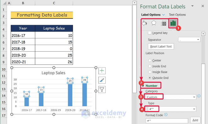
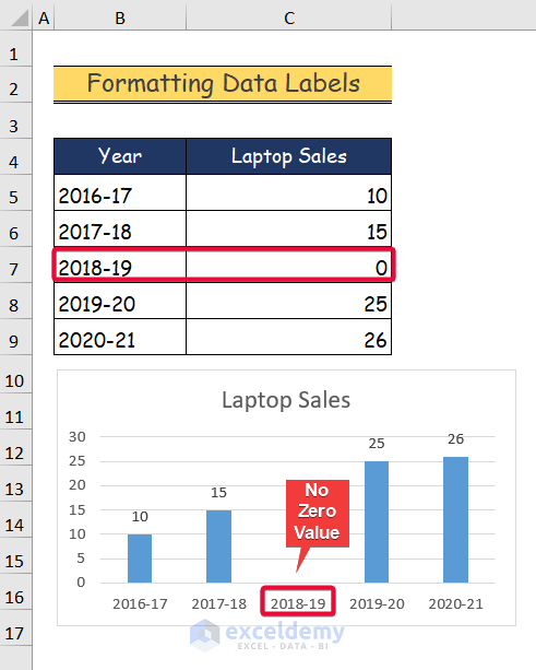
- The zero value has been removed from your chart.
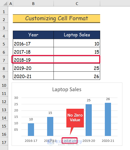
Method 3 – Customizing the Cell Format to Hide Zero Values
Steps:
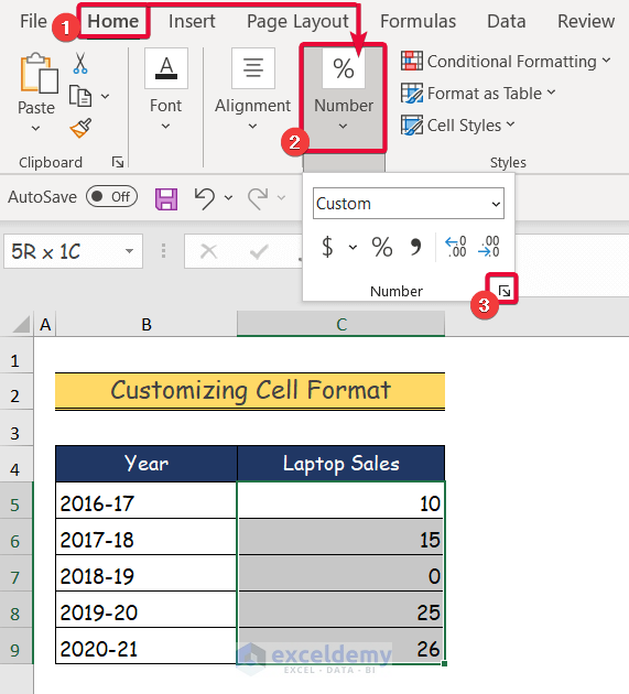
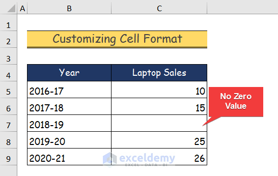
- Select the dataset containing the zero value.
- Go to the Home tab.
- Go to the Number group.
- Click on the small arrow sign to the right bottom corner of the group. The Format Cells dialogue box will appear on the screen.
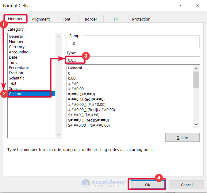
- From the Format Cells dialogue box, select the Number tab.
- Choose the Custom option.
- Insert the following under Type:
0,0;;;- Click OK.
- The zero value will vanish from your dataset.
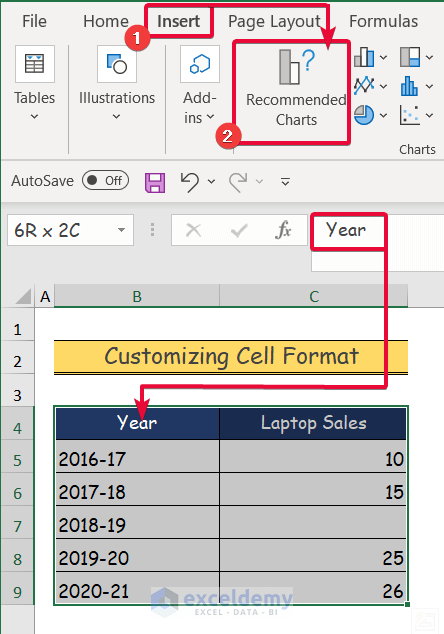
- Select the entire dataset.
- Click on the Insert tab.
- Navigate down to the Chart option.
- From the Chart group, click on the Recommended Charts tab.
- Choose a chart of your choice. We will select the Cluster Column chart.
- Click OK.
- The graph will be included in our dataset.

- Right-click on the graph.
- Pick Add Data Labels from the menu of choices.
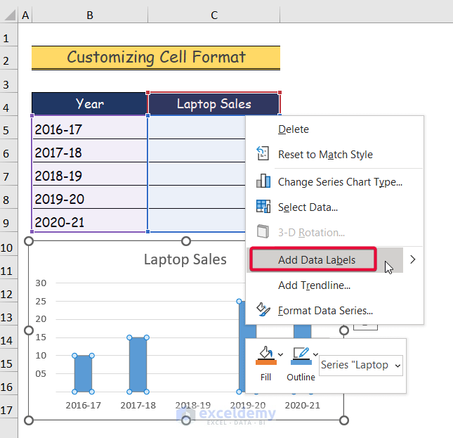
- The chart does not contain any zero value.
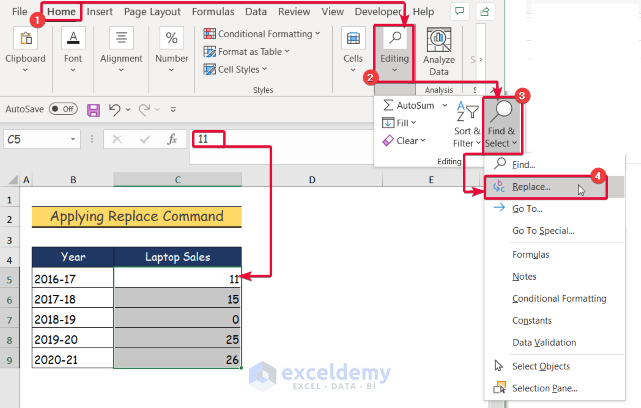
Method 4 – Applying the Replace Command to Hide Zero Values in an Excel Chart
Steps:
- Select the dataset containing the zero value.
- Go to the Home tab and the Editing group.
- Click on the Find & Select tab.
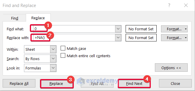
- From the drop-down options, select the Replace command. The Find and Replace dialogue box will be on the screen.
- In the dialogue box, input 0 in the Find what box.
- Put the following in the Replace with box:
=NA()- Click Replace.
- Click on the Find Next tab.
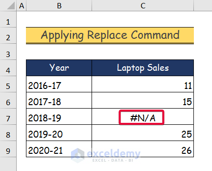
- Continue until the zero value is replaced by the NA function.
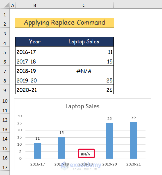
- The zero value is replaced by #N/A.
- Choose the entire dataset.
- Select the Insert tab.
- Go down to the Chart group and select the Recommended Charts option.
- Choose the chart of your choice from the recommended charts. We will choose the Cluster Column chart.
- Click OK.

- Right-click on the chart.
- Select Add Data Labels.
- The #N/A value is added in place of the zero value.
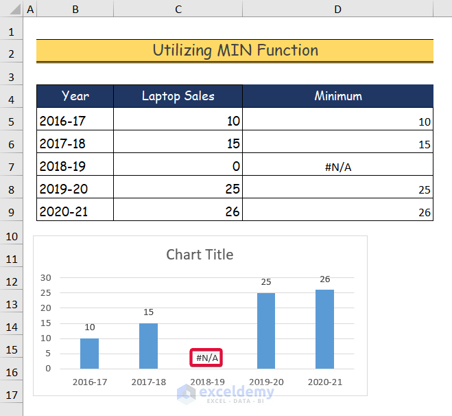
Method 5 – Use the MIN Function to Hide Zero Values
Steps:
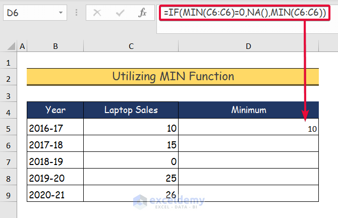
- Select the D5 cell and insert the following formula
=IF(MIN(C5:C5)=0,NA(),MIN(C5:C5))- Hit Enter.
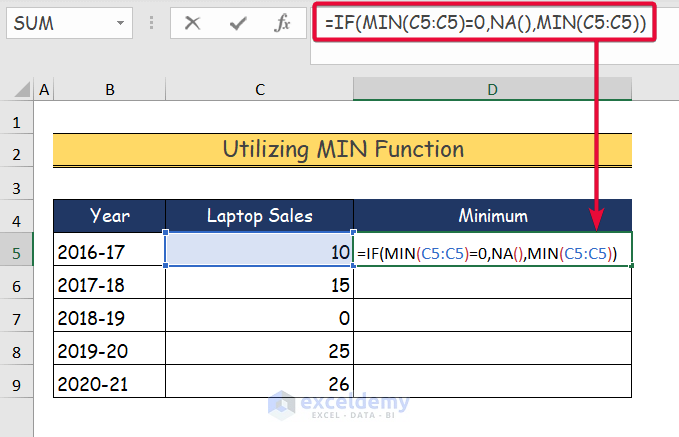
- The minimum value is added to the cell.
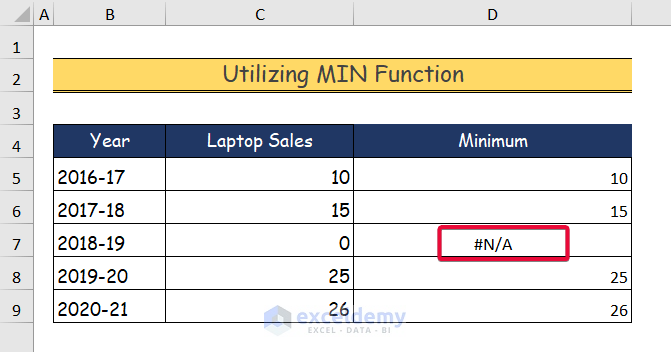
- Move the cursor down to the last data cell.
- The #N/A value will be added in place of the zero value.
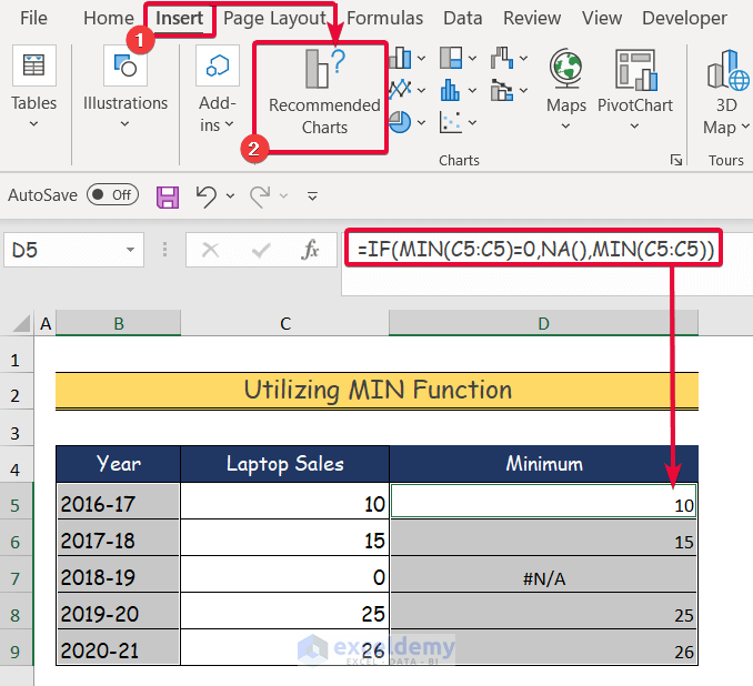
- Select the first and the last column of the dataset.
- Click on the Insert tab.
- Select the Recommended Charts option from the Chart group.
- We will select the Custer Column chat. You can choose any chart.
- Select OK.

- Right-click on the chart representing our dataset.
- From the list available, select Add Data Labels.
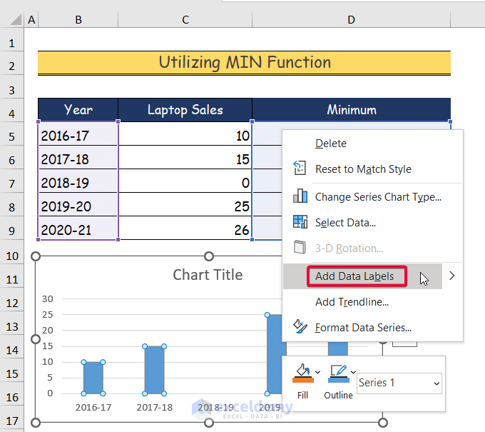
- The zero value in our chart is replaced by #N/A.
Download the Practice Workbook
Related Articles
- How to Change Decimal Places in Excel Graph
- How to Mirror Chart in Excel
- How to Resize Chart Area Without Resizing Plot Area in Excel
<< Go Back to Customize Excel Charts | Excel Charts | Learn Excel
Get FREE Advanced Excel Exercises with Solutions!

And how to how to hide blank/ zero values from a graph in excel second axis?
I want to how to hide blank/ zero values from a graph in excel but in a serie that is in the second axis. How can I do that?
Hello Daniel. You can do this by using the Find & Replace feature of Excel. From the Home tab >> under Editing group >> go to Find & Select option >> choose Replace. Then you will see the Find and Replace dialog box. Write 0 in Find what box >> write =NA() in Replace with box >> press in Find Next button >> if the cell has 0 value then press Replace button >> otherwise press Find Next.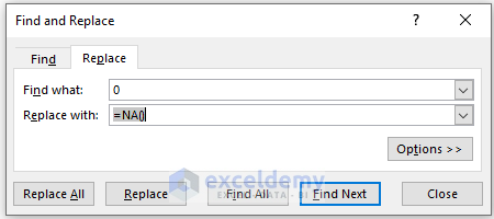
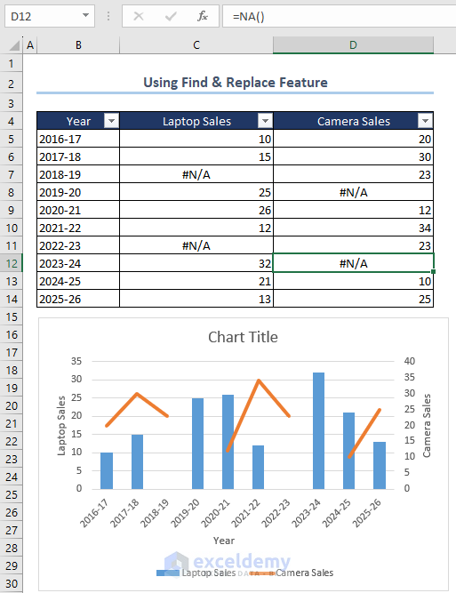
In this way change all the 0 values into =NA(). Don’t press Replace All as there may have numeric 0 with the numbers.
Now insert your chart. You will get both the axis have no zero values. Below, I have attached an image where I used two axis and remove zero value from both axis.
If you still face any problem then please provide us your worksheet in Exceldemy Forum.
No.
When I choose the data to plot in the secondary axis, the zeros continue appearing.
See: https://prnt.sc/ZiMHb7ILcOP8
Here you must use IFERROR function to get blank cell for null values. Again, you need to apply formula like if there is no data then the date will be blank also.
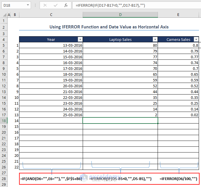
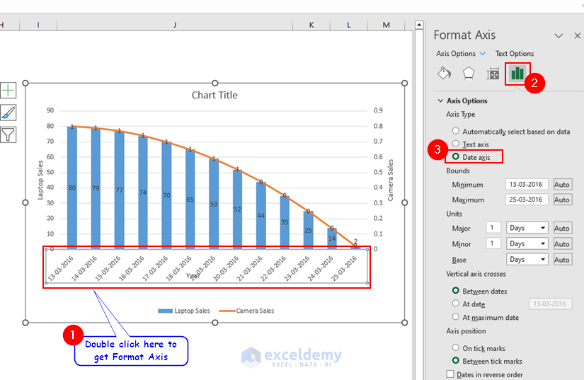
You must use Date format as Horizontal axis. Then you will get the chart auto updated up to valued cells. Double-click on Horizontal axis >> from Format Axis window (right side of Excel sheet) >> Axis Options >> Axis Type >> check Date axis.