How to Hide Notes in Excel: 3 Handy Approaches

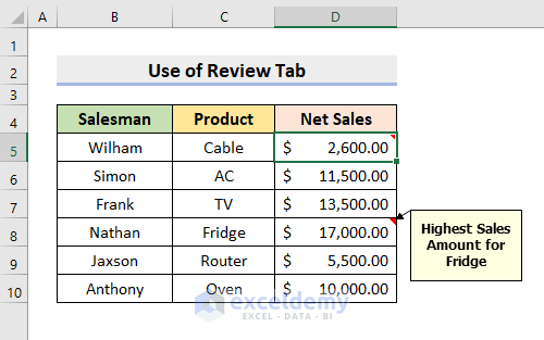
Method 1 – Hiding Notes in Excel Through Review Tab

1.1 Hiding All Notes

STEPS:

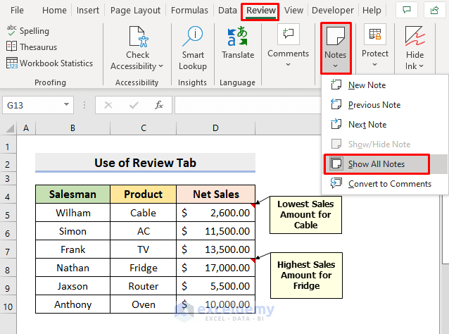
• Go to Review ➤ Notes.
• Select Show All Notes.

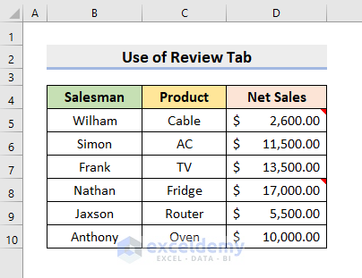
• All the notes will disappear from the worksheet.
• You’ll see your dataset as shown in the following picture.

1.2 Hiding Specific Note

STEPS:

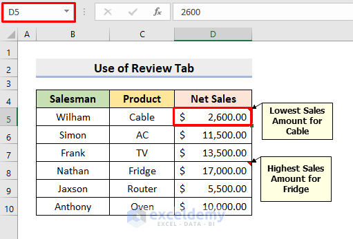
• Select the cell with the note that you want to hide.
• Select cell D5.

• Go to the Review tab.
• Choose Notes ➤ Show/Hide Note.

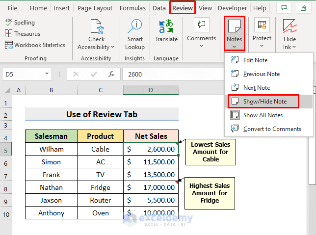
• You won’t see the D5 cell’s Note, you can see the note indicator. When you hover over the cell, only then the note will appear.

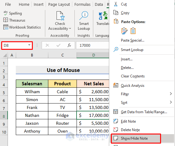
Method 2 – Using Context Menu to Hide Notes in Excel

STEPS:

• Select cell D8 at first.
• Right-click on the Mouse.
• Get a series of options to choose from.
• Click Show/Hide Note.

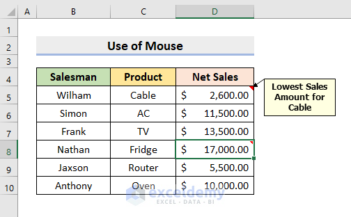
• Hide that specific note only.
• The dataset will appear like it’s demonstrated in the following image.

Method 3 – Hiding Notes Through Excel File Options

STEPS:

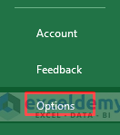
• Go to the File tab.
• In the File window, select Options.

• The Excel Options dialog box will pop out.
• Go to the Advanced tab.
• In the Display section, you’ll see 3 options for the cells with comments (For cells with comments, show).
• Check the circle for Indicators only, and comments and notes on hover.
• Choose other options according to your requirements.

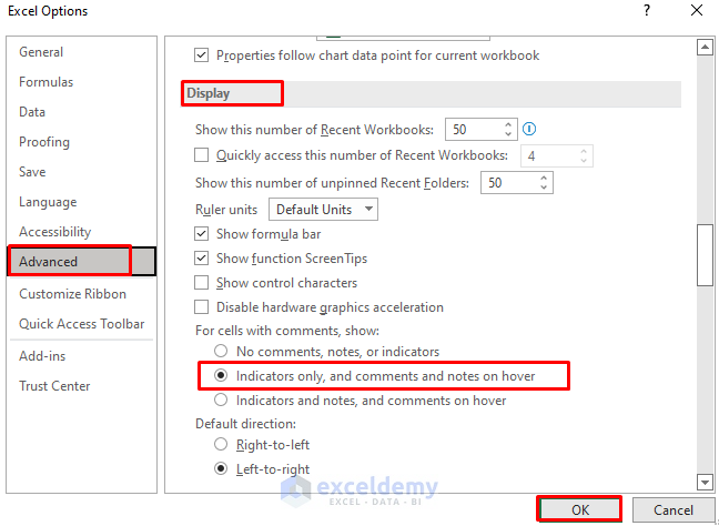
• Press OK.
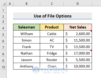
• It’ll return the worksheet and the dataset as displayed below.

Download Practice Workbook

Download the following workbook to practice by yourself.

Related Articles

• How Do I Stop My Notes from Moving in Excel
• How to Print Notes in Excel
• How to Remove Notes in Excel

<< Go Back to Notes in Excel | Learn Excel