How to Hide Gridlines on Part of a Sheet in Excel (2 Quick Ways)

By default, Excel shows gridlines in every worksheet. But we can turn it off or hide it partially if we need to. Excel has some features that we can use to do that. You will learn two quick ways from this article to hide gridlines in Excel on part of a sheet with sharp steps and clear images.

What Are Gridlines in Excel?

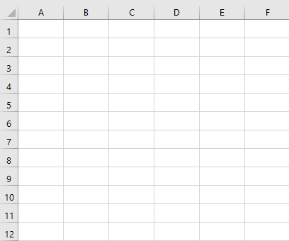
Excel uses vertical and horizontal gray lines to differentiate between cells in an organized way so that we can easily understand cells, navigate through cells, and relate the data between cells, those lines are called gridlines. Look at the image below to understand gridlines.

How to Hide Gridlines on Part of a Sheet in Excel: 2 Methods

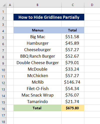
Before learning the methods, get introduced to our dataset that represents some first food item’s cost. Our worksheet contains gridlines, we’ll remove them partially- will remove them from the menu names area. Actually, there’s no direct gridline command to hide gridlines in Excel partially. So we’ll have to apply alternative tricky ways.

1. Changing Fill Color to Hide Some Selected Gridlines in Worksheet

Firstly, we’ll use the Fill Color option of Excel to hide gridlines in Excel on part of a sheet. If we select the white fill color for the specific range then the gray-colored gridlines will be placed under the white fill color of the cells and it will seem that the gridlines have gone away. We can do that following two ways.

1.1. Using Ribbon

In the Font section of the Home ribbon, there are options to change the font, fill color, text color, etc. We’ll use the Fill Color command from here.

Steps:

First, select the specific sheet area and click on the Home ribbon.
Then from the Font section, click on the drop-down icon of the Fill Color command.
Different types of theme colors will appear, choose the white color.

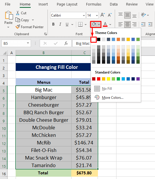
After that, the gridlines of that area will disappear because of the white fill color.

1.2. Using Right-Click

After selecting the area if we right-click our mouse then some frequently needed options of the Home ribbon will appear, where we’ll also get the Fill Color command.

Steps:

Select the area from where you want to remove gridlines.
Next, right-click your mouse, and then from the appeared menu, click on the drop-down icon of the Fill Color command.
Finally, just select the white color from the color template.

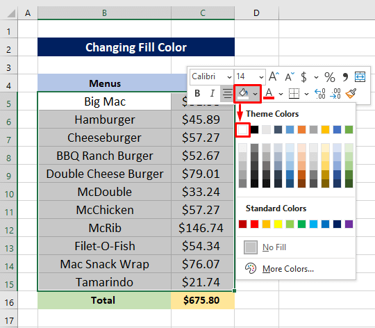
Now see, we got the same output as before.

2. Changing Border Color to Hide Some Gridlines on Part of a Sheet

If we apply borders in our dataset and then change the border color to white, then the gray gridlines will go under the white borders so, it will look like there are no gridlines. Have a look at our dataset, we have applied outside and inside borders to it. Let’s make them white.

Steps:

Select the area from where you want to remove gridlines. We selected the menu names area.
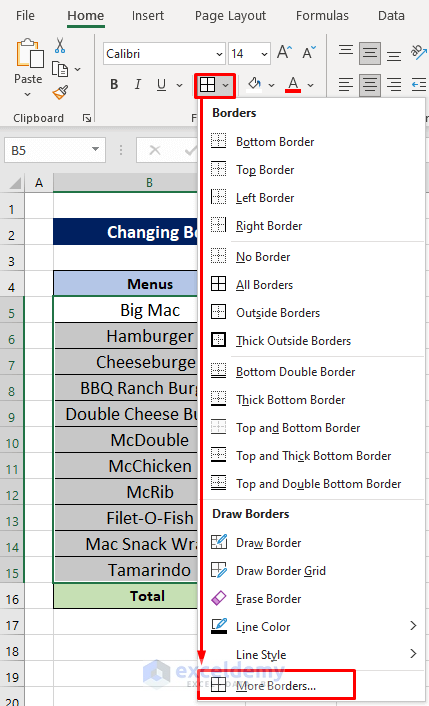
Later, click on the drop-down icon of the Borders command from the Font section of the Home ribbon.
Then select More Borders from the list.

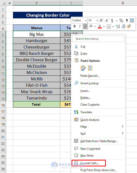
There’s another way too, right-click your mouse on the selected range.
Then choose the Format Cells option from the context menu.

A few moments later, we’ll get the Format Cells dialog box and it will take you to the Border section directly.

Then from the Border section, click on the drop-down icon of the Color box.
Next, select the white color.
Later, from the Presets part, click on the Outline and Inside options.
Finally, just press OK.

Look, the border color of that part has been changed to white color and so it hid the gridlines.

How to Remove Gridlines Using Shortcut Keys

Excel offers a lot of shortcut key combinations to do some specific tasks very first. We know how to hide gridlines in Excel by following the regular ways but there’s a shortcut key combination to remove gridlines from a whole worksheet too. The shortcut is- ALT + W, V, G.

Steps:

First, press and hold the ALT key.
Then click serially the W, V, and G

After a while, you will see that the gridlines are removed from the sheet.

How to Hide Gridlines While Printing in Excel

As gridlines are quite helpful while working in Excel you may want to keep them in your worksheet always. On the other hand, you may not want to keep it on your printed sheet. It’s quite bothering to hide the gridlines every time before printing. To overcome this situation, excel has a smart feature in the Page Layout ribbon. If we unmark that option then Excel will always print the sheet without the gridlines.

Steps:

From the Page Layout ribbon, go to the Sheet Options section.
Then just unmark the Print option from the Gridlines part.

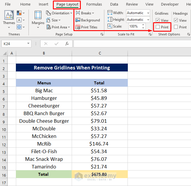
Now see the print preview, there are no gridlines, although our worksheet still contains gridlines.

Download Practice Workbook

You can download the free Excel workbook from here and practice independently.

Hide Gridlines Partially.xlsx

Conclusion

That’s all for the article. I hope the procedures described above will be good enough to hide gridlines in Excel on part of a worksheet. Feel free to ask any question in the comment section and please give me feedback.