How to Handle More Than 1048576 Rows in Excel

By default, Microsoft Excel does not allow us to work with more than 1048576 rows of data but we can analyze more than that using the Data Model feature in Excel.

Step 1 – Setting up the Source Dataset

The source dataset for this article has three columns: “Name”, “Sales”, and “Zone”.

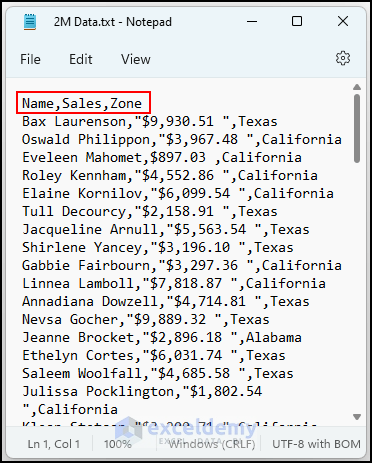
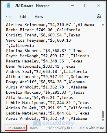
There are 2,00,001 lines (or rows) in the dataset including the heading row.

Step 2 – Importing Source Dataset

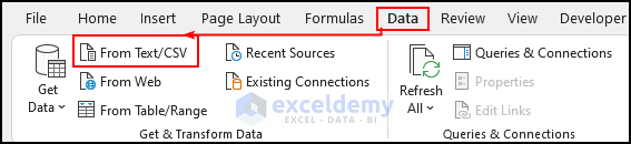
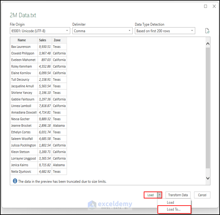
From the Data tab → select From Text/CSV.

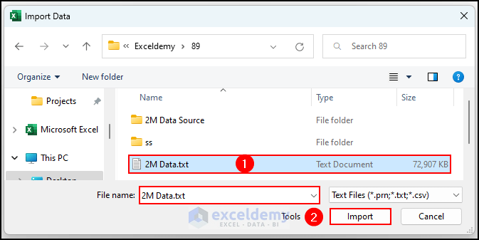
Select the downloaded source dataset from OneDrive.
Press Import.

Step 3 – Adding to the Data Model

Another dialog box will appear.
Select “Load To…”

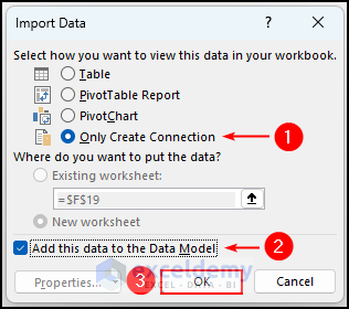
Select “Only Create Connection”.
Select “Add this data to the Data Model”.
Press OK.

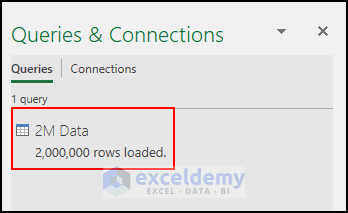
The status will state 2,000,000 rows loaded.

Step 4 – Inserting PivotTable from the Data Model

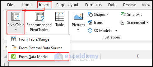
Now, utilizing the information from the Data Model, we added a pivot table.

From the Insert tab select PivotTable and from the dropdown menu select From Data Model.

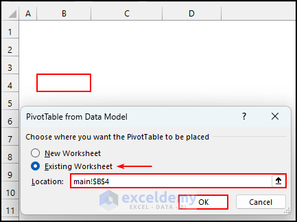
The PivotTable from the Data Model dialog box will appear.
Select Existing worksheet and specify the output.
Hit OK.

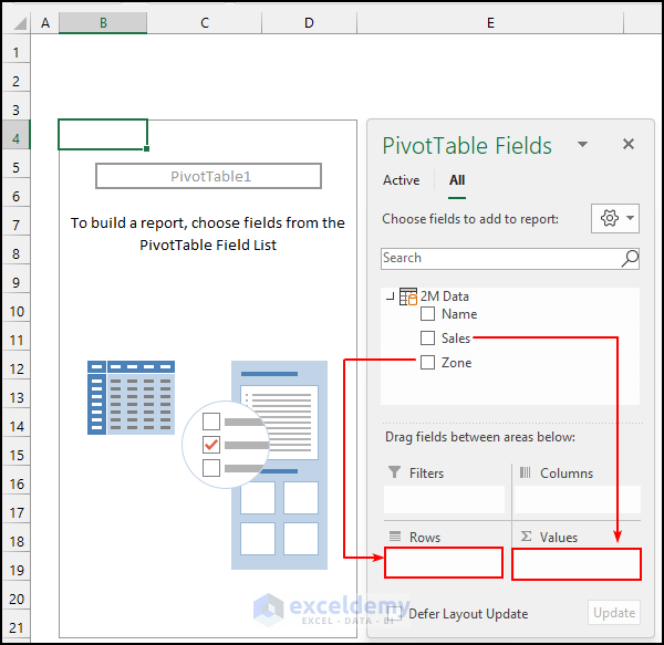
Ablank pivot table will appear.
Enter the “Zone” field in the “Row” area and the “Sales” field in the “Values” area.

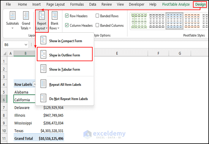
Select anywhere inside the pivot table, and from the Design tab select Report Layout.
Select Show in Outline Form. This changes Row Labels to Zone.

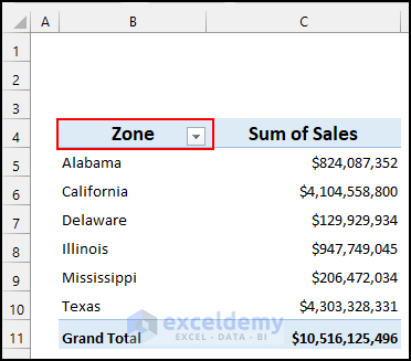
This will be the output of the pivot table.

Step 5 – Employing Slicers

Select anywhere inside the pivot table.
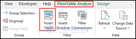
From the PivotTable Analyze tab select Insert Slicer.

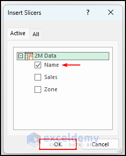
The Insert Slicers dialog box will appear.
Select Name and press OK.

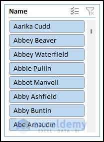
The Name Slicer will appear.

Step 6 – Inserting Charts

Select anywhere inside the pivot table.
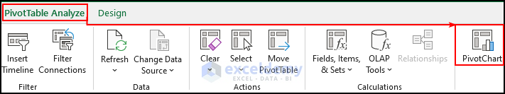
From the PivotTable Analyze tab select PivotChart.

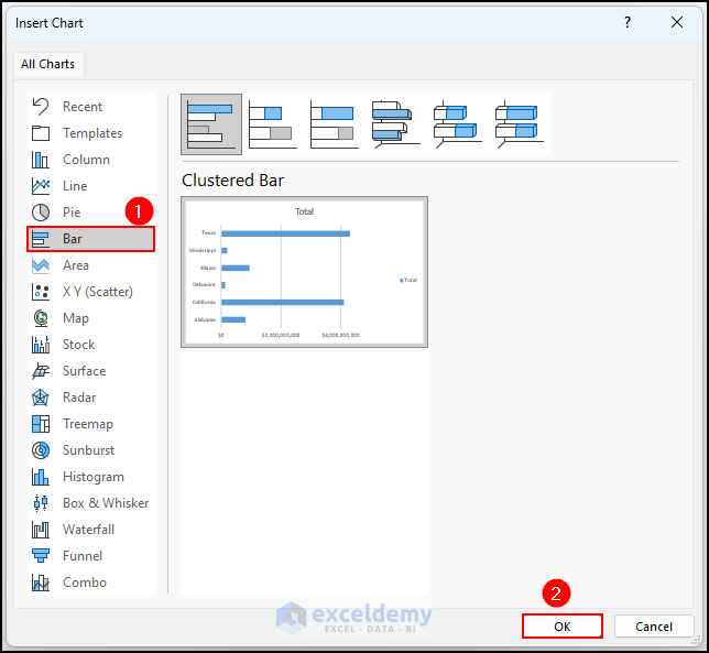
The Insert Chart box will appear.
Select Bar and press OK.

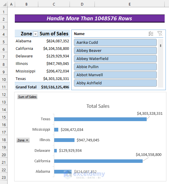
A graph has been created.

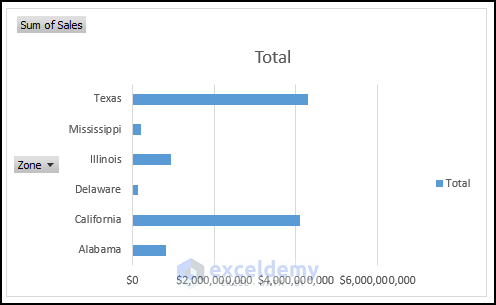
Add a title and modify the graph to suit the users needs.

Things to Remember

The Excel Data Model feature is available starting with Excel 2013. The data is kept in the computer’s memory. Therefore, if you have a slow computer, it will take a lot of time to analyze a large number of rows.

Download Practice Workbook

Handle More Than 1M Rows.xlsx