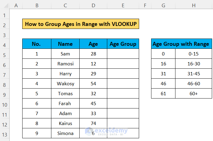
Suppose you have a dataset of 9 persons of different ages and want to put them inside particular age groups.
Step 1 – Create a List of Age Ranges
- Create a dataset and make a separate table where the age ranges are listed. Put the lower end of each group separately in a column, as noted on the image below.
Step 2 – Apply the VLOOKUP Formula
- Apply the following formula into the result cell (E5 in the sample):
=VLOOKUP(D5,$G$5:$H$9,2,1)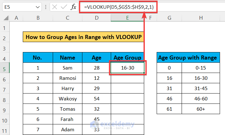
- Use the Fill handle icon to drag the formula to the other cells of the column.
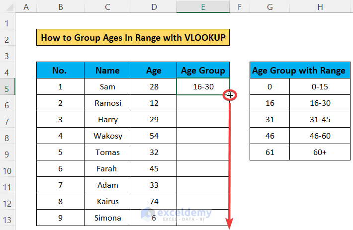
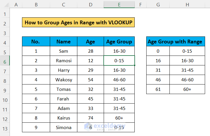
- You have got the Age Group column filled with the age groups for the cell in the Age column.
Formula Explanation:
The formula, we have used to group ages in range with the Excel VLOOKUP function is:
- =VLOOKUP(D5,$G$5:$H$9,2,1)
The Syntax of the VLOOKUP function is:
- =VLOOKUP(lookup_value,table_array,col_index_num,[range_lookup])
Lookup_value = D5:
It is a required value that it looks for in the leftmost column of the given table which can be a single value or an array of values.
So, it will look for the value of cell D5 in the leftmost column of the table. As a result, here, it will look for “28” in the 1st Column of the “Age Group with Range” table.
Table_array= $G$5:$H$9:
It is a required value which is the table where to look for the lookup_value in the leftmost column.
So, G5:H9 is the table of “Age Group with Range”. Here, you have to use absolute reference so you can copy and paste the formula into other cells keeping the table range fixed.
Col_index_num = 2:
It is also a required value which is the number of the column in the table from which a value is to be returned.
So, here the value 2 will result like it will return the value from the second column of the selected table.
[range_lookup] = 1:
It is an optional value that tells whether an exact or partial match of the lookup_value is required. Here put 0 for an exact match and 1 for a partial match. In addition, the Default is 1 (partial match).
So, here the value 1 will result in a partial match.
In the partial match, VLOOKUP takes the nearest smaller value from the list. So, for cell D5 where the value is 28 and the closest smaller value of 28 in the table is 16. As a result, it has taken the range 16-30.
Read More: How to Calculate Age in Excel from ID Number
Download the Practice Workbook
Related Articles
- How to Calculate Retirement Age in Excel
- Metabolic Age Calculator in Excel
- How to Calculate Average Age in Excel
<< Go Back to Calculate Age | Date-Time in Excel | Learn Excel
Get FREE Advanced Excel Exercises with Solutions!
