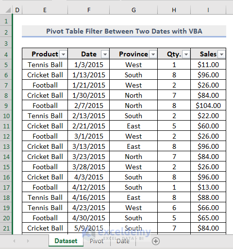
Suppose we have a huge dataset but we just want the data between two specific dates. Filtering a Pivot Table with VBA is an effective, quick, and safe method to accomplish this. In this article, we will demonstrate how to filter between two dates in this way.
How to Create a Pivot Table in Excel
There are some very good articles on Exceldemy on how to make a pivot table, how to create a pivot table using shortcuts, how to create a pivot chart in Excel and many more. But for the purpose of this article, we will briefly describe how to create a Pivot Table in Excel.
Below is the table from which we will create Pivot Tables.
Steps to Create a Pivot Table:
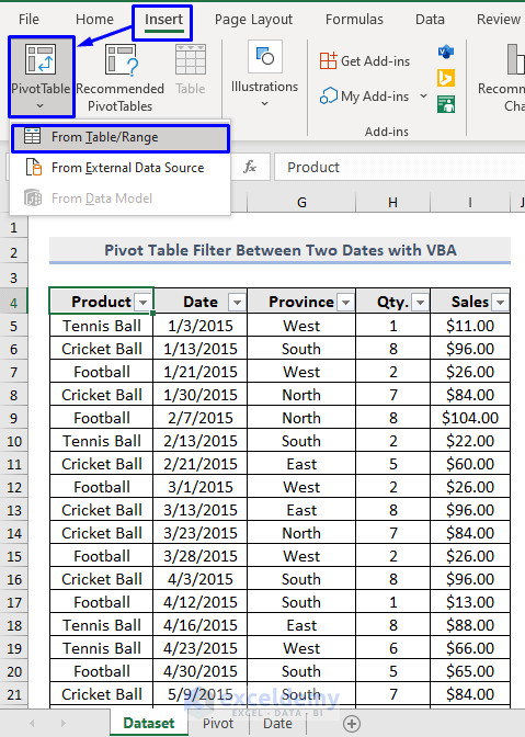
- Select any cell in the table.
- Click on the Insert tab.
- Select PivotTable -> From Table/Range.
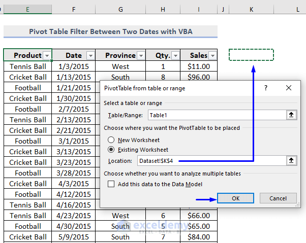
A pop-up box will appear. The whole range of the table, or if you named your table then the name of the table (in our case, Table1), will automatically appear in the Table/Range section of the box.
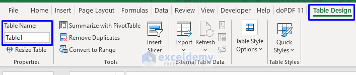
To define a name for a table:
-
- Select the whole table.
- Click on the Table Design tab.
- In the Table Name field, provide a name for the table (in our case, Table1).
Let’s continue creating the Pivot Table.
- After selecting the table or range, provide a destination for the new pivot table. To store the new pivot table in a new worksheet, check New Worksheet. Or, to store the pivot table in the same worksheet, check Existing Worksheet.
It is best practice to store the pivot table in a new worksheet, but we will store it in the same worksheet here so that it is easier to compare the source table and the pivot table.
- In the Location field, simply select the cell from where you want to start storing the pivot table. The sheet name and the cell reference number will automatically be input in the Location box. In our case, the sheet name is Dataset, and the destination cell is K4.
- Click OK.
Here is the output after creating a pivot table in cell K4.
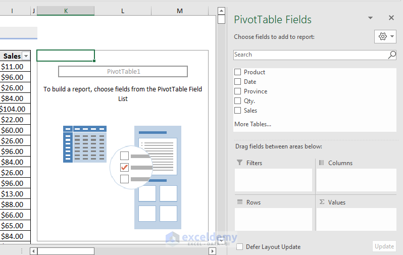
- From here, create as many pivot tables as you want by dragging and dropping the fields from above to the areas below.
Some tips in designing pivot tables:
-
- Usually, the hierarchies or the grouping fields go into the Columns area.
- The non-numeric fields fall into the Rows area.
- And the numeric fields go into the Values area.
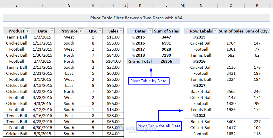
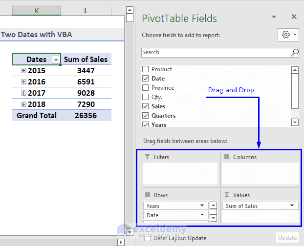
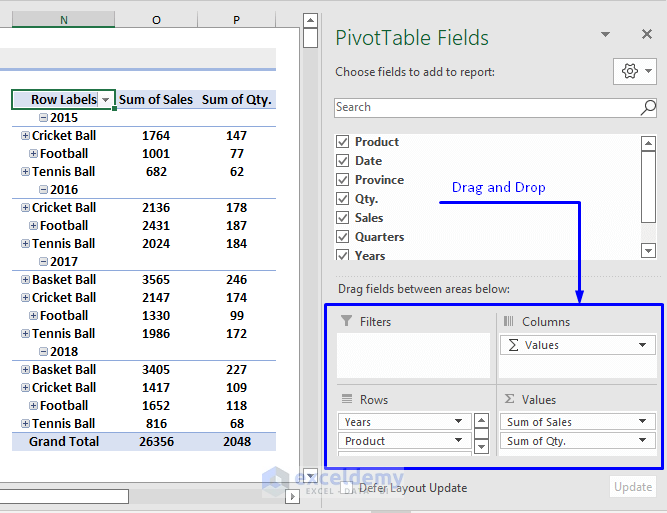
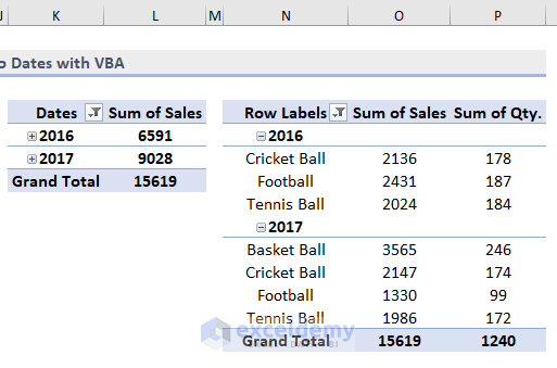
Here, we created two pivot tables, one with only Dates and Sales, and another with all the data that we have in the source table.
The stripped down table is to help illustrate what happens in the final pivot table when we start filtering. As the final pivot table usually becomes crowded with lots of data, its easier to explain using a more minimal pivot table.
Let’s assign some meaningful names to the pivot tables:
- Click on the first cell of the table.
- Click on the PivotTable Analyze tab.
- In the field named PivotTable Name in the PivotTable group, provide an appropriate name for the table (we used PvtByDate).
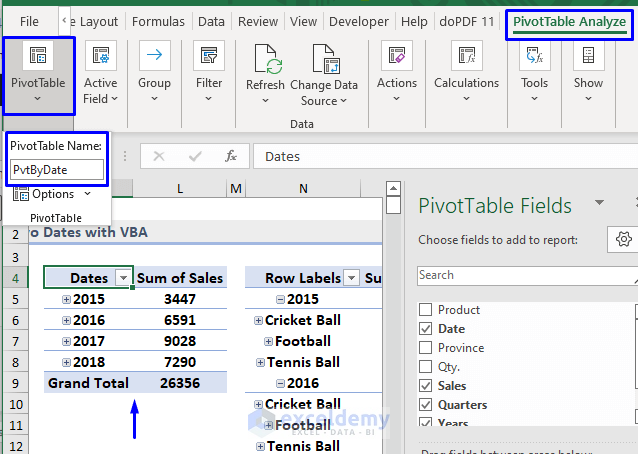
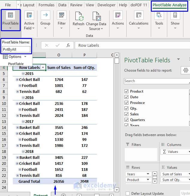
For the pivot table created with all the values, we gave the name PvtByAll.
Here is an overview of the pivot tables created:
- For the PvtByDate table:
- All the dates and related fields – Years, Quarters, Months – go into the Rows area.
- Numeric values such as Sales fall into the Values area.
- For the PvtByAll table:
- All the dates and related fields – Years, Quarters, Months – go into the Rows. The non-numeric values such as Product and Province also fall into this area.
- Numeric values such as Sales and Qty go into the Values area.
We have finished creating the pivot tables from the source table.
Now, let’s filter between two dates in these pivot tables with VBA code.
Using a VBA Macro to Filter Between Two Dates in Pivot Tables
Our approach here is to enable simply clicking a button to filter between two dates in our pivot tables. Input the two dates, click the button, and the data in the spreadsheet will automatically be filtered accordingly. We’ll use a VBA Macro to accomplish this.
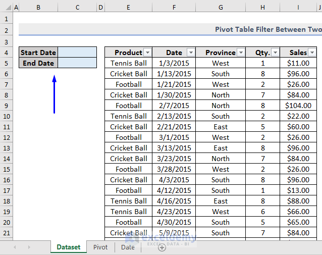
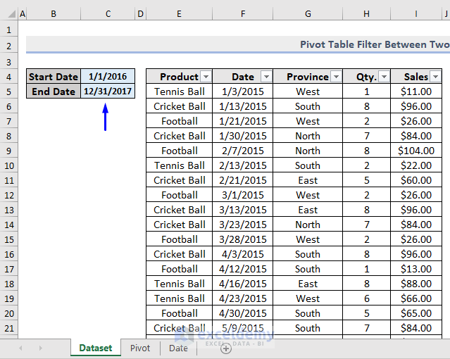
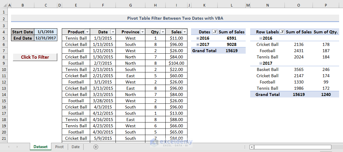
Let’s assign the two dates in our dataset.
- As in the image below, store the Start Date in cell C4 and End Date in cell C5.
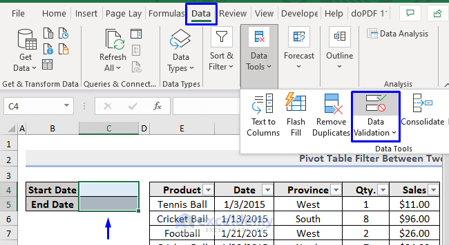
Before storing the dates, we’ll apply Data Validation to those cells, so that if invalid dates are entered in those cells, Excel will return warning messages.
- To apply Data Validation:
- Select cells C4 and C5.
- Go to tab Data.
- Select Data Validation from the Data Tools group.
-
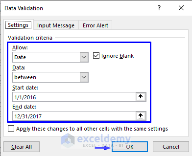
- In the Data Validation pop-up box that appears:
- Pick Date for the Allow criteria.
- Select between for the Data criteria.
- Provide a start date (in our case, 1/1/2016) and end date (12/31/2017) in the Start date and End date criteria fields respectively.
- In the Data Validation pop-up box that appears:
-
- Click OK.
Now we can safely store the required date values in those cells.
- Enter the start date (1/1/2016) value in cell C4 and end date (12/31/2017) value in cell C5.
Now let’s create the button we’ll click to filter the pivot tables for entries between the dates we just entered.
Steps to Create a Button to Filter Between Two Dates in the Pivot Table:
- To assign a button in our dataset, go to the Developer tab.
- Click Insert and select Button from the Form Controls group.
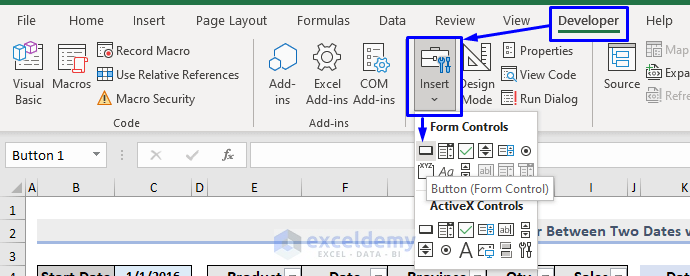
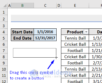
A plus symbol (+) will appear as in the image below.
- Drag the symbol to create a button of any size anywhere in your spreadsheet.
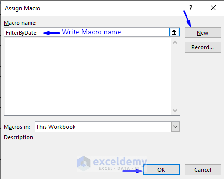
After dragging, a box named Assign Macro will pop up.
- Enter the Macro name that you want to run when the button is clicked. In our case, we name the macro as FilterByDates.
- Click New, as it is a new VBA macro.
- Click OK.
An auto-generated VBA code window will open.
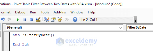
- Copy the following code and paste it into the code window:
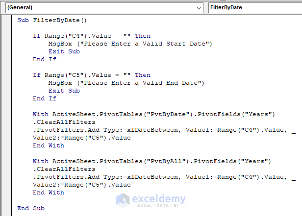
Sub FilterByDate()
If Range("C4").Value = "" Then
MsgBox ("Please Enter a Valid Start Date")
Exit Sub
End If
If Range("C5").Value = "" Then
MsgBox ("Please Enter a Valid End Date")
Exit Sub
End If
With ActiveSheet.PivotTables("PvtByDate").PivotFields("Years")
.ClearAllFilters
.PivotFilters.Add Type:=xlDateBetween, Value1:=Range("C4").Value, Value2:=Range("C5").Value
End With
With ActiveSheet.PivotTables("PvtByAll").PivotFields("Years")
.ClearAllFilters
.PivotFilters.Add Type:=xlDateBetween, Value1:=Range("C4").Value, Value2:=Range("C5").Value
End With
End Sub
The code is now ready to run.
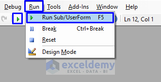
- To run the macro, either press F5 on your keyboard, select Run -> Run Sub/UserForm from the menu bar, or click on the small Run icon in the sub-menu bar.
The pivot tables now display only the filtered date values.
Instead of running the macro manually each time, because the code was written inside a button control, we can simply change the Start Date and End Date and click the button to re-filter.
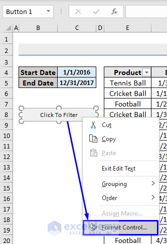
Let’s format the button.
-
- Double click on the text of the button to enable Edit mode.
- Provide a name for the button, for example Click To Filter.
- Right-click on the button and select Format Control…
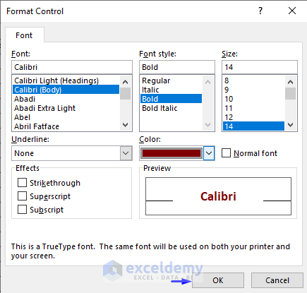
-
- In the Format Control pop-up window, modify the button as desired, for example style the text with Bold font, make the size 14, and change the font color.
- After styling the button, click OK.
Our button looks rather clickable.
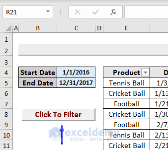
Of course, the button will still work even if it looks unappealing.
Let’s check that it works as intended. First, let’s clear the filters that were applied when we ran the macro:
- Click on the dropdown list right next to the table headers.
- Select Clear Filter From “Years”.
- Clear filters from both tables in the same way.
- Click OK.
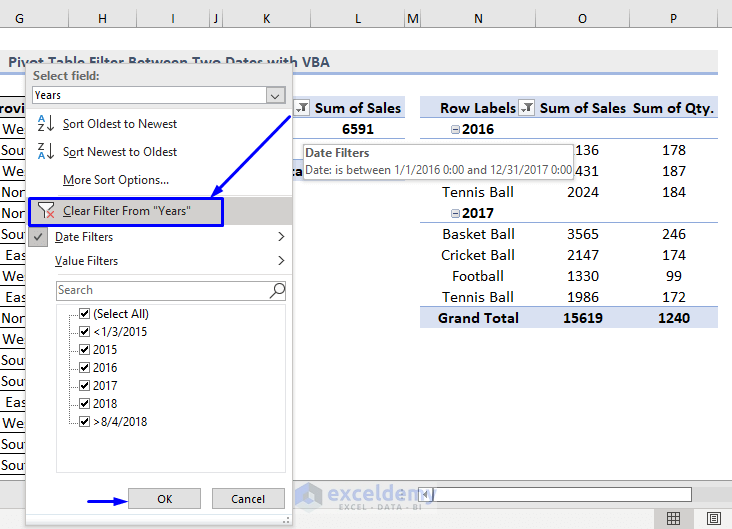
- Now, click the button.
The pivot tables are filtered according to the specified condition, namely only the dates between 1/1/2016 and 12/31/2017 are displayed.
We have successfully created pivot tables from a source table, then filtered them between two dates with VBA.
VBA Code Explanation
If Range("C4").Value = "" Then
MsgBox ("Please Enter a Valid Start Date")
Exit Sub
End If
If there is no valid date in cell C4, a warning message will be shown.
If Range("C5").Value = "" Then
MsgBox ("Please Enter a Valid End Date")
Exit Sub
End If
If there is no valid date in cell C5, a warning message will be shown.
With ActiveSheet.PivotTables("PvtByDate").PivotFields("Years")
.ClearAllFilters
.PivotFilters.Add Type:=xlDateBetween, Value1:=Range("C4").Value, Value2:=Range("C5").Value
End With
This piece of code:
- Clears all the existing filters from the PvtByDate pivot table.
- Finds the PivotFields name (“Years”) in the Rows area of the pivot table.
- Filters the dates by the Type provided here – xlDateBetween – meaning the filter will occur between dates. The date values are provided in the Value1 and Value2 variables. We pass the cell reference numbers of the start date (cell C4) and end date (cell C5) into those variables respectively.
If you don’t want to filter the PvtByDate table, omit the above piece of code. The code will then filter the PvtByAll table only.
With ActiveSheet.PivotTables("PvtByAll").PivotFields("Years")
.ClearAllFilters
.PivotFilters.Add Type:=xlDateBetween, Value1:=Range("C4").Value, Value2:=Range("C5").Value
End With
This piece of code:
- Clears all the existing filters from the PvtByDate pivot table.
- Finds the PivotFields name (“Years”) in the Rows area of the pivot table created.
- Filters the dates by the Type provided here – xlDateBetween – meaning the filter will occur between dates. The date values are provided in the Value1 and Value2 variables. We pass the cell reference numbers of the start date (cell C4) and end date (cell C5) into those variables respectively.
If you don’t want to filter the PvtByAll table, omit this piece of code. The code will then filter the PvtByDate table only.
Download Workbook
Related Articles
- Excel VBA to Filter Pivot Table Based on Multiple Cell Values
- Excel VBA to Filter Pivot Table Based on List
- How to Use Excel VBA to Filter Pivot Table
- Excel VBA to Filter Pivot Table Based on Cell Value

