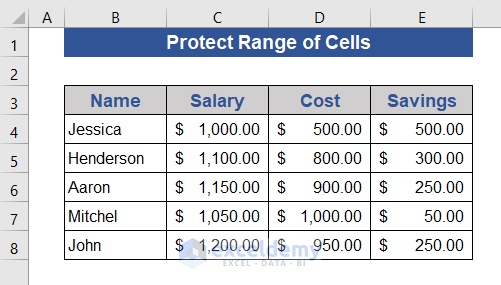
Excel VBA to Protect Range of Cells (3 Examples)

We have a dataset that contains formulas in the Savings column and the rest are values.

Method 1 – Protect a Certain Range of Cells

Steps:

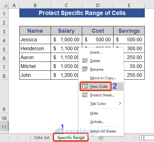
Go to the Sheet Name and right-click on it.
Choose the View Code option from the Context Menu.

In the VBA window, choose Module from the Insert tab.

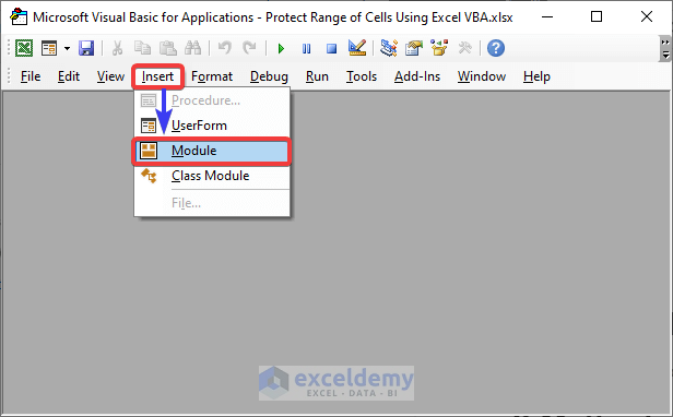
A VBA module window appears. We will write our VBA code here.

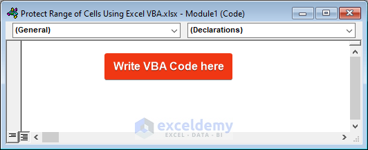
Copy and paste the following VBA code into the module.

Sub Protect_Range_Cells()
Dim range_1 As Range
Set range_1 = Range("B4:E8")
Cells.Select
Selection.Locked = False
range_1.Select
Selection.Locked = True
ActiveSheet.Protect DrawingObjects:=False, Contents:=True, Scenarios:=False
End Sub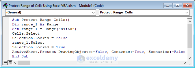

Press F5 to run the VBA code.

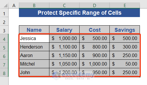
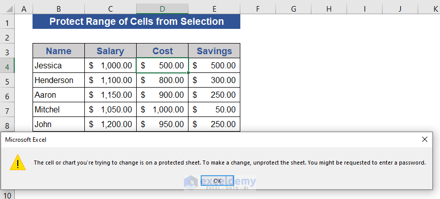
Click on any of the cells of the inputted range.

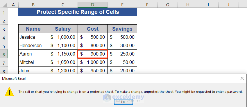
A warning shows that the cell is in protected mode. We can edit or insert data on other cells.

Code Breakdown:

Dim range_1 As Range

Declare a variable of the range type.

Set range_1 = Range("B4:E8")

Set the value of the variable.

Selection.Locked = False

Unlocks the selected range. The False comment unlocks the range.

range_1.Select
Selection.Locked = True

Selects range_1 and locks the selection.

Method 2 – Protect Cells from Selection with a Password

Steps:

Select the cells of the Cost and Savings columns of the worksheet.
Open a VBA module and insert the following VBA code.
Press the F5 button to run the code.

Sub Protect_Range_With_Pass()
 Dim pass_1 As String
 pass_1 = "Exceldemy"
 If ActiveSheet.ProtectContents = True Then
   ActiveSheet.Unprotect Password:=pass_1
 End If
 ActiveSheet.Cells.Locked = False
 Selection.Locked = True
 ActiveSheet.Protect Password:=pass_1
End Sub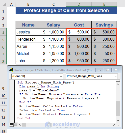

Click on any cells of the Cost or Savings columns.

A warning will show.

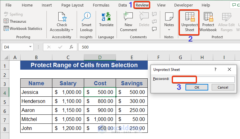
To unlock the cells, click on the Unprotect Sheet option from the Review tab.
The Unprotect Sheet window will appear.
Insert the password on the Password box and then press OK.

Code Breakdown:

Dim pass_1 As String

Declares the variable of string type.

pass_1 = "Exceldemy"

Sets a value of the variable.

If ActiveSheet.ProtectContents = True Then
ActiveSheet.Unprotect Password:=pass_1
End If

An If condition is applied. Sets the value of the pass_1 variable as the password.

ActiveSheet.Cells.Locked = False

Unlocks the active cells.

Selection.Locked = True

Locks the selected cells.

 ActiveSheet.Protect Password:=pass_1

Sets pass_1 as the password of the cells of the present sheet.

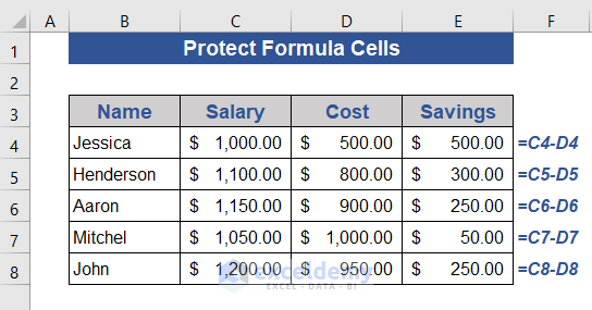
Method 3 – Detect Cells with Formulas and Protect them

We have formulas in the Savings column. We will protect those cells.

Steps:

Copy the VBA code below and paste it into a VBA module.

Sub Protect_Formula_Cells()
For Each cell In ActiveSheet.Range("B4:E8")
If cell.HasFormula Then
cell.Locked = True
Else
cell.Locked = False
End If
Next cell
ActiveSheet.Protect "abcd"
End Sub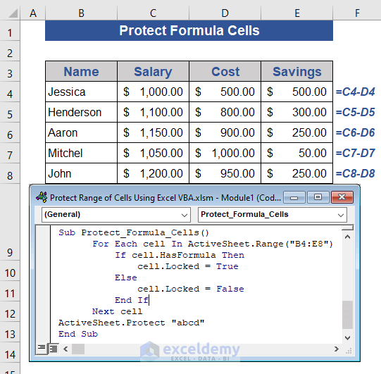

Hit the F5 button to run the code.
Click on any cells of the Savings column that contain formulas.

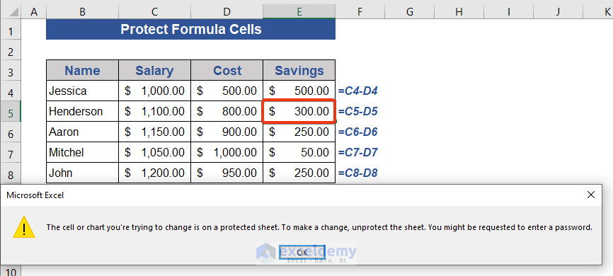
We get a warning dialog box.

Code Breakdown:

For Each cell In ActiveSheet.Range("B4:E8")

A for loop is applied on the range of the present sheet.

If cell.HasFormula Then
cell.Locked = True
Else
cell.Locked = False
End If

An If condition applied. If our selected range has any formula then those cells will be locked. And the rest of the cells will be unlocked.

ActiveSheet.Protect "abcd"

The active sheet is protected by a password.

Download the Practice Workbook

Protect Range of Cells.xlsm

Get FREE Advanced Excel Exercises with Solutions!

Sub Protect_Multiple_Range_with_Password_for_Specific_User() Dim ws As Worksheet Set ws = ThisWorkbook.Sheets("Sheet1") 'change accordingly Dim i As Integer For i = ws.Protection.AllowEditRanges.Count To 1 Step -1 ws.Protection.AllowEditRanges(i).Delete Next i ' Define the ranges and passwords rangeAddresses = Array("B5:C10", "E5:F10", "H5:I10", "K5:L10") ' Add or modify ranges as needed passwords = Array("passuser1", "passuser2", "passuser3", "passuser4") ' Add or modify passwords as needed 'Unlocking Sheet if already locked If ws.ProtectContents = True Then ws.Unprotect Password:=1234 'change accordingly End If For i = LBound(rangeAddresses) To UBound(rangeAddresses) ws.Protection.AllowEditRanges.Add Title:="Range_" & CStr(i + 1), Range:=ws.Range(rangeAddresses(i)), Password:=passwords(i) ws.Range(rangeAddresses(i)).Locked = True Next i MsgBox "Multiple ranges have been set for different users with different passwords using AllowEditRanges feature.", vbInformation 'again Locking the sheet with master password 1234 ws.Protect Password:=1234, DrawingObjects:=True, Contents:=True, Scenarios:=True End Sub

2 Comments

Tom Oct 14, 2023 at 8:39 PM

Hi,
I am wanting to make a log (using Excel) for Shift Supervisors that they can password lock their entries. Can more than 4 individuals use their own password to lock their range of cells using VBA?

Alok Paul Oct 15, 2023 at 4:51 PM

Dear Tom,
Thanks for reading our articles. Here, you queried that you want an Excel sheet based on VBA to input values for 4 users in separate specified range. Those cells are locked with different passwords for each user.
Here, we have set User 1 with range B5:C10 and password: passuser1, User 2 with range E5:F10 and password: passuser2, User 3 with range H5:I10 and password: passuser3, User 4 with range K5:L10 and password: passuser4.

Based on the above information our VBA code will be as follow.

• When you double-click on any cell specified for any user a window named Unlock Range will pop-up. Insert the password and click on OK to edit the range of the user.