How to Filter Based on Cell Value Using Excel VBA (4 Methods)

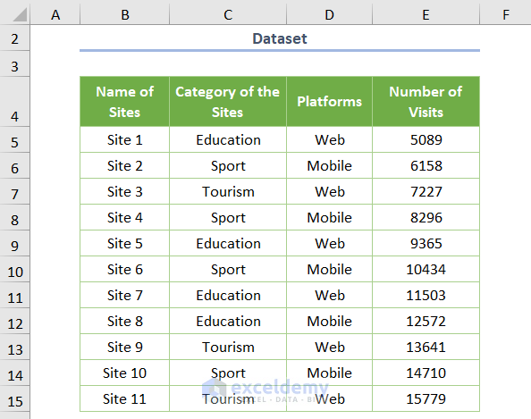
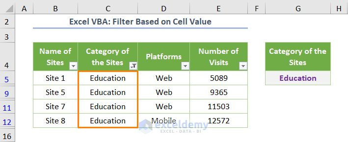
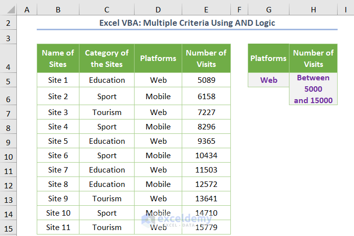
Let’s introduce today’s dataset (B4:E15 cell range) as shown in the following screenshot. Here, the Number of Visits for each website is provided along with the Name and Category of the Sites. The dates and mode of Platforms are also given. Let’s filter the table based on a specific cell value.

Method 1 – Filter Based on a Certain Cell Value

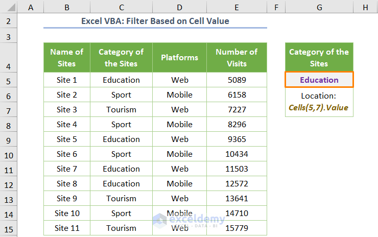
Let’s put “Education”, one of options for the Category of the Sites, in the G5 cell. We’ll use it to filter the table. That means the row number and column number of the location of the cell are 5 and 7, respectively.

Steps:

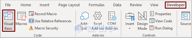
• Open a module by clicking on the Developer tab and selecting Visual Basic.

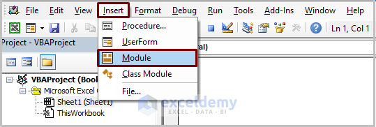
• Go to Insert and select Module.

• Inside the empty module, copy the following code:

Sub Filter_CellValue1()
ActiveSheet.Range("B4:E15").AutoFilter field:=2, Criteria1:=Cells(5, 7).Value
End Sub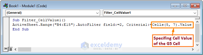

⧭ In the above code, we used the ActiveSheet property and the Range object to assign the entire dataset. Then, we used the AutoFilter method along with the field as 2 and Criteria1 as the value of the G5 cell. The value of the field is 2 since the Category of the Sites is located at the second position from the left of the dataset. We specified the value of the cell using the Cells property.

• Run the code (the keyboard shortcut is F5 or Fn + F5), and you’ll get the following filtered dataset.

Read More: Filter Multiple Criteria in Excel with VBA (Both AND and OR Types)

Method 2 – Filter Based on Cell Value Using a Drop-down List 

Steps

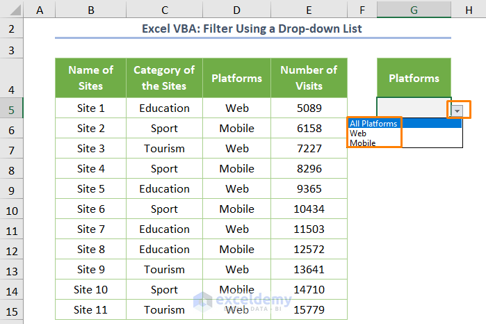
• Select the filter cell, in this case G5.
• Choose the Data Validation tool from the Data Tools ribbon in the Data tab.

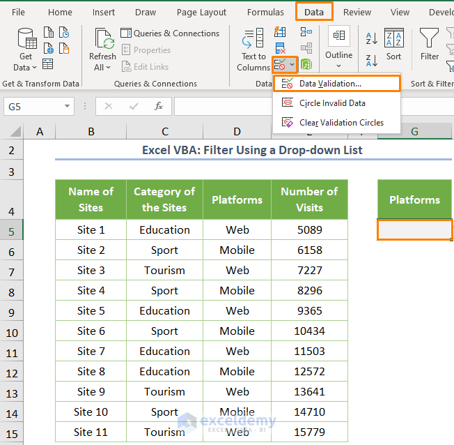
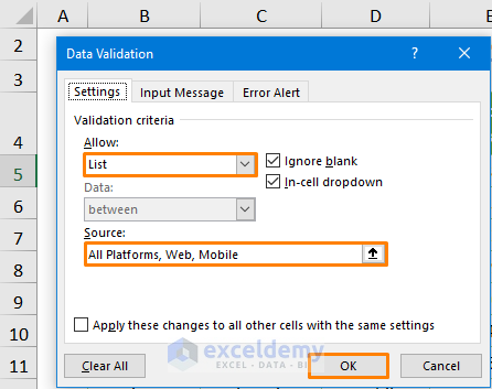
• You’ll see the following dialog box where you need to choose the List under the Allow criteria.
• Insert All Platforms, Web, Mobile in the box for Source. Alternatively, you can create a drop-down list with unique values.

• Press OK, and you’ll see the following drop-down list.

• Go to the Sheet tab of the active sheet (at the bottom) and right-click on the current sheet’s name.
• Choose the View Code option.

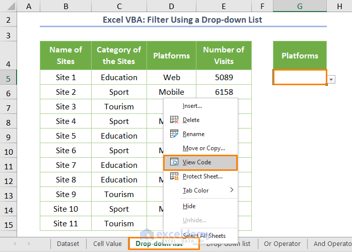
• Copy-paste the following code inside the module that opens:

Private Sub Worksheet_Change(ByVal Target As Range)
If Target.Address = "$G$5" Then
 If Range("G5").Value = "All Platforms" Then
  Range("B5").AutoFilter
 Else
  Range("B5").AutoFilter field:=3, Criteria1:=Range("G5").Value
 End If
End If
End Sub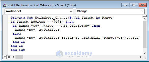

⧭ In the above code, we used the Worksheet.Change event which processes continuous changes in cell values within the worksheet. Then, we utilized the If…Then…Else statement along with the AutoFilter method to filter the dataset based on either “All Platforms” (with no criteria) or other values of the G5 cell (with criteria).

• Close the VBA Editor.
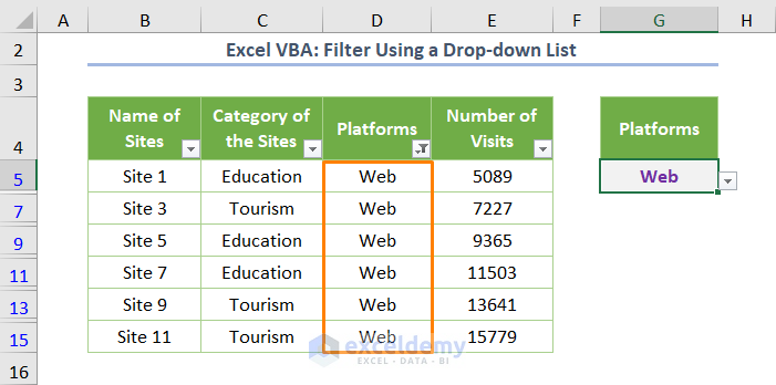
• Go to the main worksheet and choose any platform from the drop-down list.
• We chose the Web platform to filter the dataset.

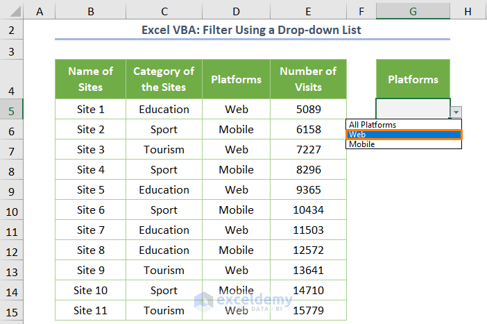
• We got the following filtered data based on the Web platform.

Read More: Excel VBA: How to Filter with Multiple Criteria in Array

Method 3 – Filter with Multiple Criteria Using the OR Operator

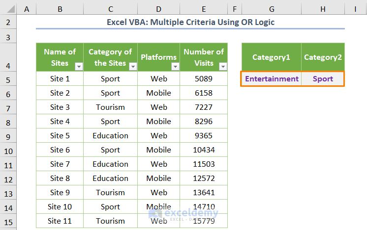
Suppose that you have two categories of the sites in the G5:H5 cell. Category1 is Entertainment which is not available along with the whole dataset and Category2 is about Sport. We’ll return results that satisfy either one of the criteria.

• Open the VBA editor (right-click on the sheet name and select View Code).
• Copy the following code:

Sub Using_OR_Logic()
Dim range_to_filter As Range

Set range_to_filter = Range("B4:E15")

range_to_filter.AutoFilter field:=2, Criteria1:=Cells(5, 7).Value, Operator:=xlOr, Criteria2:=Cells(5, 8).Value

End Sub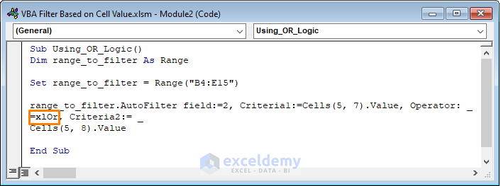

• Run the code by saving and closing the tab.

⧭ Things to Keep in Mind While Using the Above Code:

• Range: It refers to the cell range to filter e.g. B4:E15.
• Field: It is the index of the column number from the leftmost part of your dataset. The value of the second field will be 2.
• Criteria 1: The first criteria for a field e.g. Criteria1=Cells(5, 7).Value
• Criteria 2: The second criterion for a field e.g. Criteria2=Cells(5, 8).Value
• Operator: An Excel operator that specifies certain filtering requirements. Here, the Or operator is used which returns TRUE if any input is TRUE.

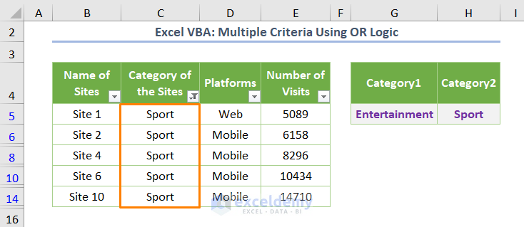
After running the code, you’ll get the filtered output based on Sport only as Category1 is not available in the dataset.

Read More: How to Remove Filter in Excel VBA

Method 4 – Multiple Criteria Using the AND Operator

If you want to filter the dataset based on specific Platforms as well as a range of the Number of Visits (let’s between 5,000 and 15,000), we need to apply the AND to make sure the cells satisfy both criteria.

• Open the VBA module and copy the following code:

Dim range_to_filter As Range

Set range_to_filter = Range("B4:E15")

range_to_filter.AutoFilter field:=3, Criteria1:=Cells(5, 7).Value, Operator:=xlAnd
range_to_filter.AutoFilter field:=4, Criteria1:=">=5000", Criteria2:="<=15000"

End Sub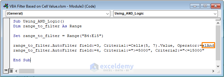

⧭ Things to Keep in Mind While Using the Above Code:

• Field: the value of the field for the Platforms is 3 and the Number of Visits is 5.
• Criteria 1 of Platforms: The first criteria for a field e.g. Criteria1=Cells(5, 7).Value
• Criteria1 and 2 of the Number of Visits: The first criteria for the field e.g. Criteria1=”>=5000”  and the second criteria is Criteria2=“<=15000” 
• Operator: here, I used the And operator which returns TRUE if all statements are TRUE. Otherwise, it will return FALSE.

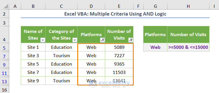
If you run the code, you’ll get the following output.

Read More: Excel VBA to Filter in Same Column by Multiple Criteria

Related Articles

• Excel VBA: Filter Based on Cell Value on Another Sheet
• Excel VBA: Filter Table Based on Cell Value
• VBA Code to Filter Data in Excel
• Filter Different Column by Multiple Criteria in Excel VBA