Excel VBA: How to Filter with Multiple Criteria in Array (7 Ways)

If you are looking for ways to filter with multiple criteria array in Excel VBA, then you are in the right place. Filtering a large dataset based on multiple criteria can be made easier with the help of VBA codes rather than using the conventional feature of Excel.
So, let’s start our main article.

Download Workbook

7 Ways to Filter with Multiple Criteria in Array Using Excel VBA

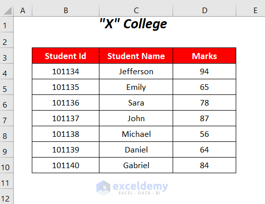
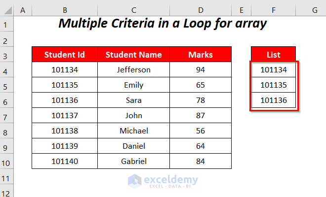
In the following dataset, we have some records of marks corresponding to the name of the students and their ids. We will try to filter this dataset based on different criteria as an array by using some codes.

We have used Microsoft Excel 365 version here, you can use any other versions according to your convenience.

Method-1: Filter with Multiple Criteria as Texts in Array

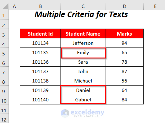
Here, we will try to filter the following dataset based on the Student Name column for multiple criteria containing the strings Emily, Daniel, and Gabriel in an array.

Step-01:
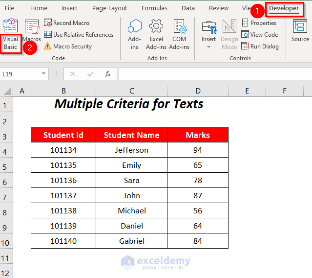
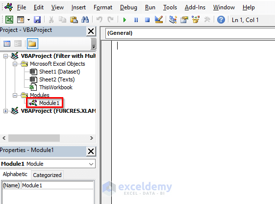
➤ Go to the Developer Tab >> Visual Basic Option.

Then, the Visual Basic Editor will open up.
➤ Go to the Insert Tab >> Module Option.

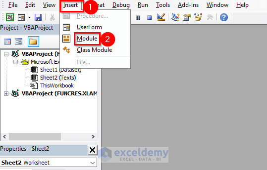
After that, a Module will be created.

Step-02:
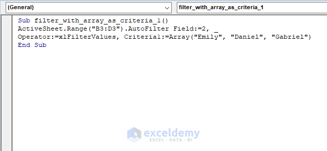
➤ Write the following code

Sub filter_with_array_as_criteria_1()

ActiveSheet.Range("B3:D3").AutoFilter Field:=2, _
Operator:=xlFilterValues, Criteria1:=Array("Emily", "Daniel", "Gabriel")

End Sub

Here, we declared the header names in the range B3:D3 in which we will apply the filter and Field:=2 is the column number of this range based on which we will do this filtering process.
Finally, we have set the criteria as an array for declaring multiple students’ names such as Emily, Daniel, and Gabriel.

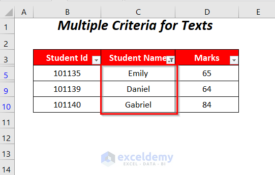
➤ Press F5.
Then, you will have the dataset filtered down for multiple criteria to show the name of the students and their corresponding Ids and Marks for the students Emily, Daniel, and Gabriel.

Read More: Filter Multiple Criteria in Excel (4 Suitable Ways)

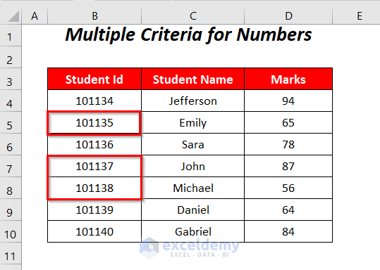
Method-2: Filter with Multiple Number Criteria in Array Using Excel VBA

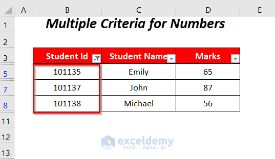
Here, we will be filtering down the following dataset for the ids 101135, 101137, and 101138 by using these numbers as multiple criteria in an array.

Steps:
➤ Follow Step-01 of Method-1.
➤ Write the following code

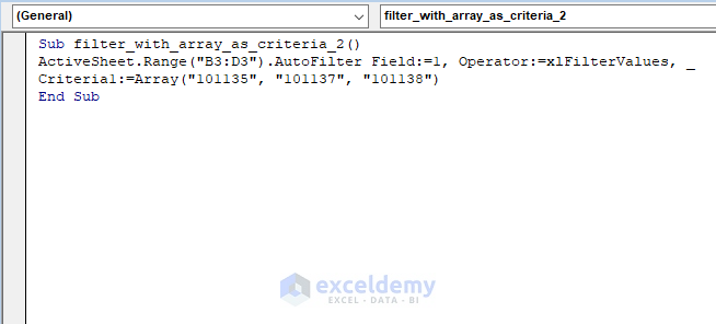
Sub filter_with_array_as_criteria_2()

ActiveSheet.Range("B3:D3").AutoFilter Field:=1, Operator:=xlFilterValues, _
Criteria1:=Array("101135", "101137", "101138")

End Sub

Here, we declared the header names in the range B3:D3 in which we will apply the filter and Field:=2 is the column number of this range based on which we will do this filtering process.
Finally, we have set the criteria as an array for declaring multiple students’ ids such as 101135, 101137, and 101138 and we have put them inside inverted commas to specify them as strings because AutoFilter will work for only an array of strings.

➤ Press F5.
After that, you will get the names and marks of the students having ids 101135, 101137, and 101138.

Read More: VBA to Get Unique Values from Column into Array in Excel (3 Criteria)

Method-3: Setting Multiple Criteria in a Range for Using as Array

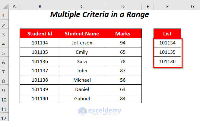
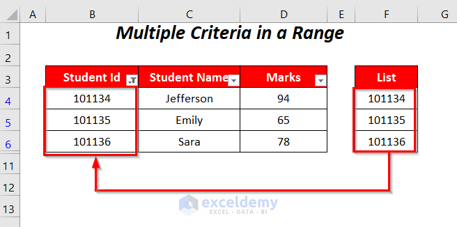
Here, we have listed the criteria in the List column containing the ids 101134, 101135, and 101136 based on which we will do our filtering process.

Steps:
➤ Follow Step-01 of Method-1.
➤ Write the following code

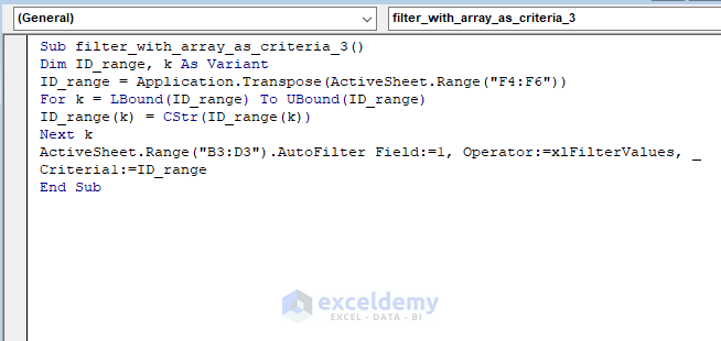
Sub filter_with_array_as_criteria_3()

Dim ID_range, k As Variant
ID_range = Application.Transpose(ActiveSheet.Range("F4:F6"))

For k = LBound(ID_range) To UBound(ID_range)
ID_range(k) = CStr(ID_range(k))
Next k
ActiveSheet.Range("B3:D3").AutoFilter Field:=1, Operator:=xlFilterValues, _
Criteria1:=ID_range

End Sub

Here, we have declared ID_range, k as Variant and ID_range is the array that will store multiple criteria, and k is the increment ranging from the lower limit to the upper limit of this array. For having the lower limit and upper limit we used the LBOUND function and UBOUND function respectively.
The FOR loop is used for converting the values other than strings in the array into strings with the help of the CStr function. Finally, we have utilized this array as Criteria1.

➤ Press F5.
Afterward, you will get the names and marks of the students having ids 101134, 101135, and 101136.

Read More: Filter Different Column by Multiple Criteria in Excel VBA

Similar Readings

• How to Filter Unique Values in Excel (8 Easy Ways)
• Perform Custom Filter in Excel (5 Ways)
• Calculate the Average of an Array with VBA (Macro, UDF, and UserForm)
• Shortcut for Excel Filter (3 Quick Uses with Examples)

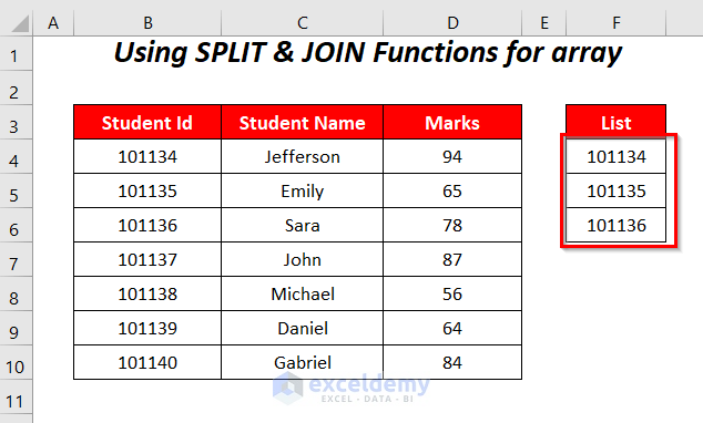
Method-4: Using SPLIT and JOIN Functions for Creating Array with Multiple Criteria

Here, we will utilize the following list in the List column as an array and for filtering the dataset properly we will also use the SPLIT function, JOIN function, and TRANSPOSE function in a VBA code.

Steps:
➤ Follow Step-01 of Method-1.
➤ Write the following code

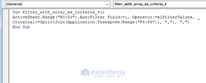
Sub filter_with_array_as_criteria_4()

ActiveSheet.Range("B3:D3").AutoFilter Field:=1, Operator:=xlFilterValues, _
Criteria1:=Split(Join(Application.Transpose(Range("F4:F6")), ","), ",")

End Sub

Here, TRANSPOSE will convert the 2D array into a 1D array otherwise AutoFilter will not work, JOIN will join each of the values into an array of strings, and finally, SPLIT will break down each string to give input them separately as criteria for filtering the dataset.

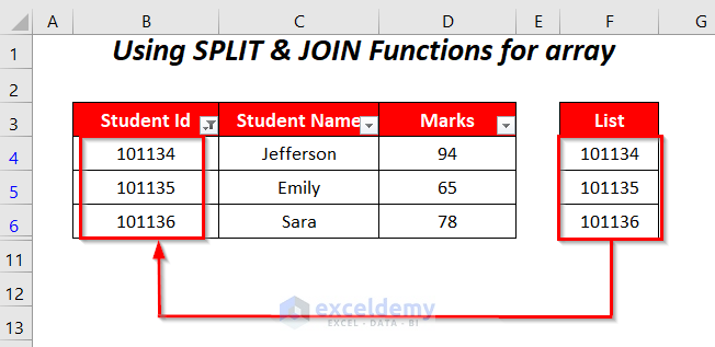
➤ Press F5.
Finally, you will get the names and marks of the students having ids 101134, 101135, and 101136.

Read More: How to Split a String into an Array in VBA (3 Ways)

Method-5: Filter with Multiple Criteria in a Loop for Array with VBA

In this section, we will be filtering down the following dataset depending on the Student Id column for multiple criteria as listed in the List column.

Steps:
➤ Follow Step-01 of Method-1.
➤ Write the following code

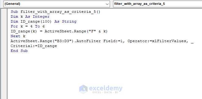
Sub filter_with_array_as_criteria_5()

Dim k As Integer
Dim ID_range(100) As String

For k = 4 To 6
ID_range(k) = ActiveSheet.Range("F" & k)
Next k
ActiveSheet.Range("B3:D3").AutoFilter Field:=1, Operator:=xlFilterValues, _
Criteria1:=ID_range

End Sub

Here, we have declared k as Integer, ID_range(100) as String where ID_range is an array that will store up to 100 values. To determine the values for this array here we have used the FOR loop for k from 4 to 6 as the row numbers of the List column and F is the column name.
Finally, we have used this array as Criteria1 for AutoFilter.

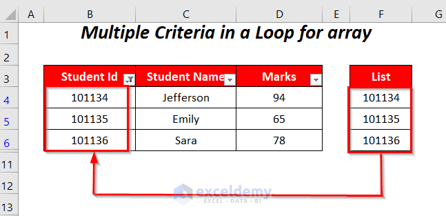
➤ Press F5.
Eventually, you will get the names and marks of the students having ids 101134, 101135, and 101136.

Read More: Filter Multiple Criteria in Excel with VBA (Both AND and OR Types)

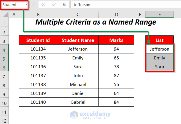
Method-6: Using Named Range for Multiple Criteria

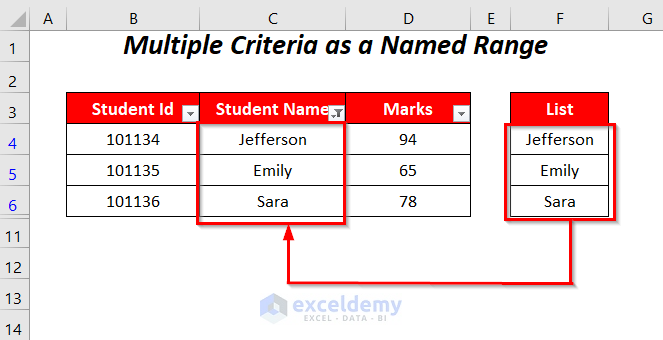
Here, we have listed some names of the students in the List column and named this range as Student. Using this named range we will define an array that will contain multiple criteria for the AutoFilter feature.

Steps:
➤ Follow Step-01 of Method-1.
➤ Write the following code

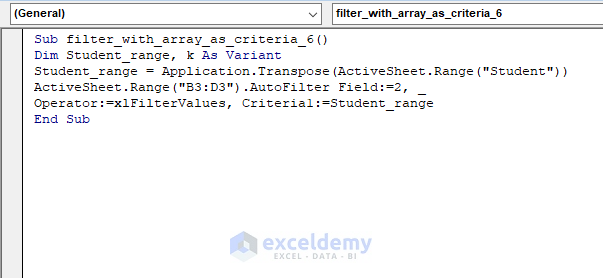
Sub filter_with_array_as_criteria_6()

Dim Student_range, k As Variant
Student_range = Application.Transpose(ActiveSheet.Range("Student"))
ActiveSheet.Range("B3:D3").AutoFilter Field:=2, _
Operator:=xlFilterValues, Criteria1:=Student_range

End Sub

Here, we have declared Student_range, k as a Variant, and used the TRANSPOSE function to convert the 2D array of the named range Student into a 1D array and then stored it in Student_range. Then, it is used as Criteria1 for the AutoFilter method.

➤ Press F5.
Then, you will have the dataset filtered down for multiple criteria to show the name of the students and their corresponding Ids and Marks for the students Jefferson, Emily, and Sara.

Related Content: VBA to Transpose Array in Excel (3 Methods)

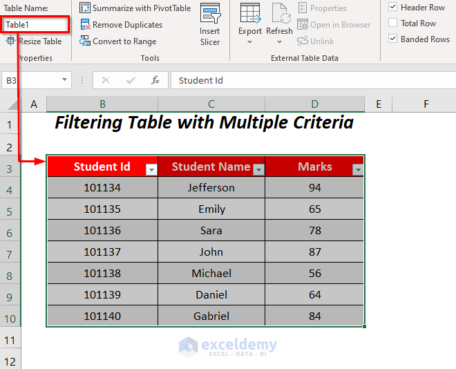
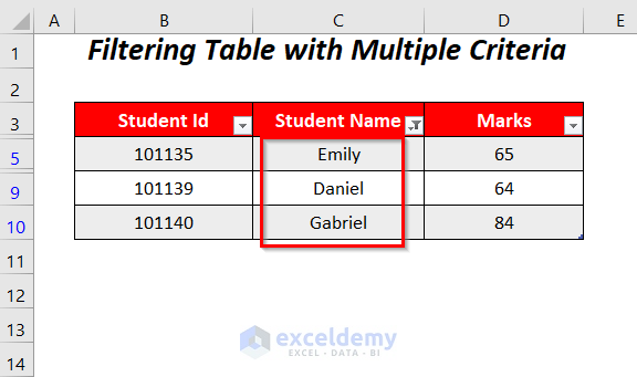
Method-7: Filter Table with Multiple Criteria in an Array

Here, we have the following Table whose name is Table1 and using Excel VBA we will try to filter down this table based on the names Emily, Daniel, and Gabriel as multiple criteria in an array.

Steps:
➤ Follow Step-01 of Method-1.
➤ Write the following code

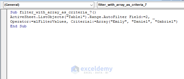
Sub filter_with_array_as_criteria_7()

ActiveSheet.ListObjects("Table1").Range.AutoFilter Field:=2, _
Operator:=xlFilterValues, Criteria1:=Array("Emily", "Daniel", "Gabriel")

End Sub

Here, ListObjects(“Table1”) is used for defining the table Table1, Field:=2 for setting up the second column of this range as a base of the filtering process and finally we have defined an array containing multiple names for Criteria1.

➤ Press F5.
Eventually, you will have the dataset filtered down for multiple criteria to show the name of the students and their corresponding Ids and Marks for the students Emily, Daniel, and Gabriel.

Read More: Excel VBA: Filter Table Based on Cell Value (6 Easy Methods)

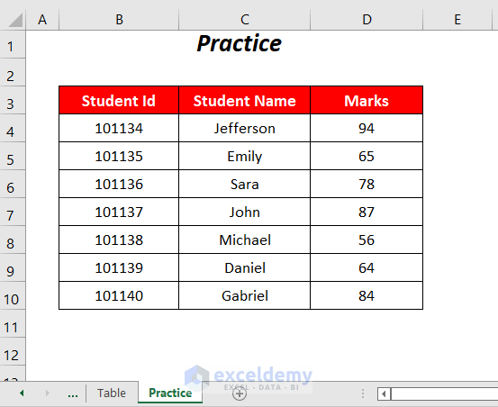
Practice Section

For doing practice by yourself we have provided a Practice section like below in a sheet named Practice. Please do it by yourself.

Conclusion

In this article, we tried to cover the ways to filter with multiple criteria as an array using Excel VBA easily. Hope you will find it useful. If you have any suggestions or questions, feel free to share them in the comment section.

Related Articles

• How to Remove Filter in Excel VBA (5 Simple Methods)
• ReDim Preserve 2D Array in Excel VBA (2 Easy Ways)
• How to Filter Based on Cell Value Using Excel VBA (4 Methods)
• Excel VBA to Create Data Validation List from Array
• How to Convert Range to Array in Excel VBA (3 Ways)
• Excel VBA to Filter in Same Column by Multiple Criteria (6 Examples)
• How to Name a Table Array in Excel (With Easy Steps)