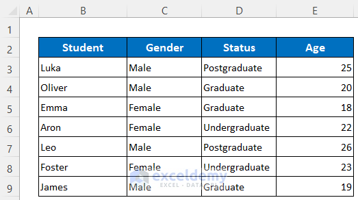
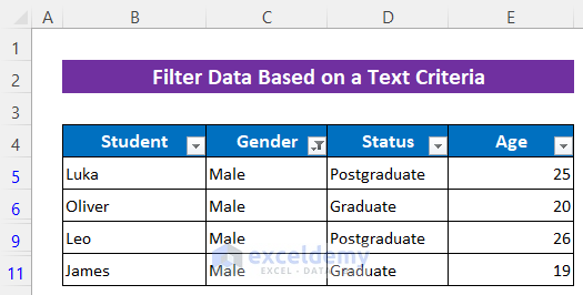
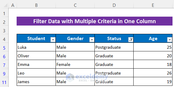
The following dataset contains students’ Gender, Status, and Age.
Example 1 – Using a VBA Code to Filter Data Based on Text Criteria in Excel
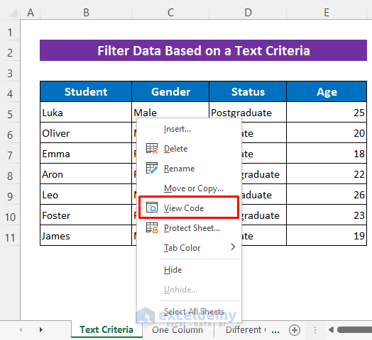
Steps:
A VBA window will open.
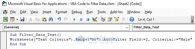
- Enter the following code.
Sub Filter_Data_Text()
Worksheets("Text Criteria").Range("B4").AutoFilter Field:=2, Criteria1:="Male"
End Sub- Minimize the VBA.
Code Breakdown
- A Sub procedure, Filter_Data_Text() is created.
- The Range property declares sheet name and range
- The AutoFilter method uses the Criteria: Field:=2 means column 2. Criteria1:=”Male” to Filter data for Male.
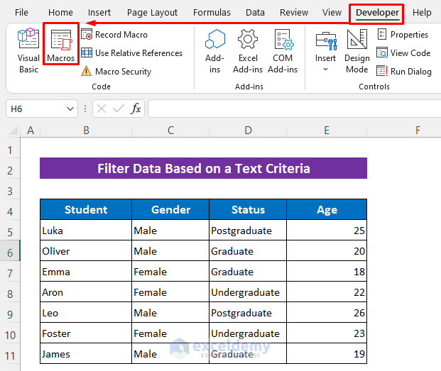
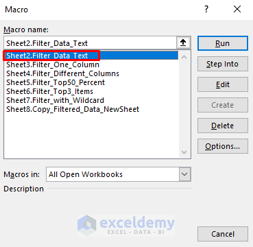
- Select the Macro name.
- Click Run.
This is the output.
Example 2 – Applying a VBA Macro to Filter Data with Multiple Criteria in One Column
Steps:
- Follow the two first steps in Example 1 to open the VBA window.
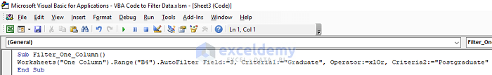
- Enter the following code.
Sub Filter_One_Column()
Worksheets("One Column").Range("B4").AutoFilter Field:=3, Criteria1:="Graduate", Operator:=xlOr, Criteria2:="Postgraduate"
End Sub- Minimize the VBA.
Code Breakdown
- A Sub procedure, Filter_One_Column(), is created.
- The Range property declares our sheet name and range
- The AutoFilter method uses the Criteria: Field:=3 means column 3. Here, Criteria1:=”Graduate” and Criteria2:=”Postgraduate” to Filter the student’s Status.
- The Operator:=xlOr function applies the OR condition Filter for multiple criteria.
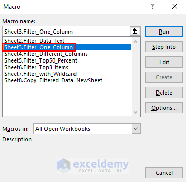
- Follow the third step in Example 1 to open the Macros dialog box.
- Choose the selected Macro and click Run.
This is the output.
Read More: Filter Multiple Criteria in Excel with VBA (Both AND and OR Types)
Example 3 – Applying a VBA code to Filter Data with Multiple Criteria in Different Columns
Steps:
- Follow the first two steps in Example 1 to open the VBA
- Enter the following code.
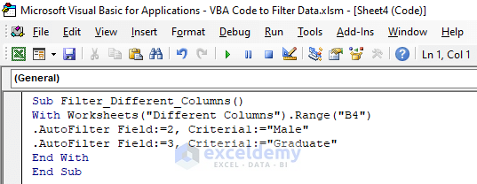
Sub Filter_Different_Columns()
With Worksheets("Different Columns").Range("B4")
.AutoFilter Field:=2, Criteria1:="Male"
.AutoFilter Field:=3, Criteria1:="Graduate"
End With
End Sub- Minimize the VBA window.
Code Breakdown
- A Sub procedure, Filter_Different_Columns() is created.
- The With statement uses Multiple Column.
- The Range property declares sheet name and range.
- The AutoFilter method uses the Criteria: Field:=2 means column 2 and Field:=3 means column 3.
- Selects Criteria1:=”Male” for the Gender column and Criteria1:=”Graduate” for the Status column to Filter data from different columns.
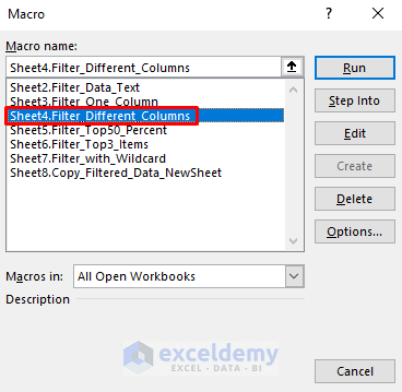
- Follow the third step in Example 1 to open the Macros dialog box.
- Choose the selected Macro and click Run.
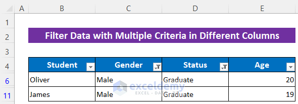
This is the output.
Read More: How to Filter Based on Cell Value Using Excel VBA
Example 4 – Using a VBA Code to Filter the Top 3 Items in Excel
Steps:
- Follow the two first steps in Example 1 to open the VBA window.
- Enter the following codes.
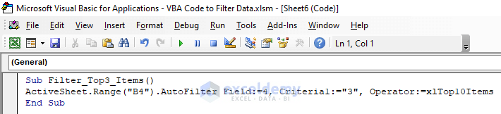
Sub Filter_Top3_Items()
ActiveSheet.Range("B4").AutoFilter Field:=4, Criteria1:="3", Operator:=xlTop10Items
End Sub- Minimize the VBA window.
Code Breakdown
- A Sub procedure, Filter_Top3_Items() is created.
- The Operator:=xlTop10Items is used to Filter for the top three data.
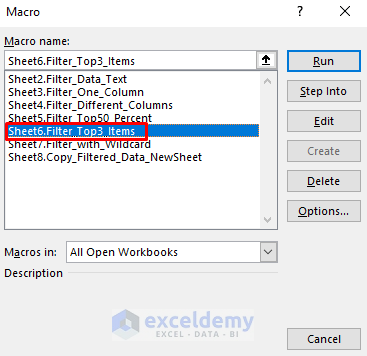
- Follow the third step in Example 1 to open the Macros dialog box.
- Select the Macro and click Run.
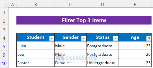
This is the output.
Read More: Excel VBA: How to Filter with Multiple Criteria in Array
Example 5 – Applying a VBA Code to Filter the Top 50 Percents in Excel
Steps:
- Follow the two first steps in Example 1 to open the VBA window.
- Enter the following code.
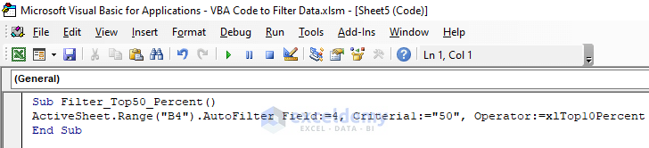
Sub Filter_Top50_Percent()
ActiveSheet.Range("B4").AutoFilter Field:=4, Criteria1:="50", Operator:=xlTop10Percent
End Sub- Minimize the VBA window.
Code Breakdown
- A Sub procedure, Filter_Top50_Percent() is created.
- Operator:=xlTop10Percent is used to Filter the top fifty percent in column-4.
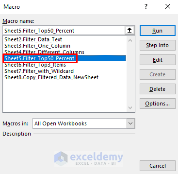
- Follow the third step in Example 1 to open the Macros dialog box.
- Select the Macro and click Run.
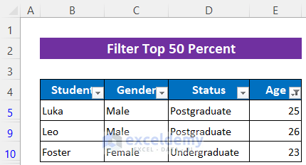
This is the output.
Read More: How to Remove Filter in Excel VBA
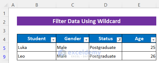
Example 6 – Applying a VBA Code to Filter Data Using the Wildcard
Steps:
- Follow the two first steps in Example 1 to open the VBA window.
- Enter the following code.
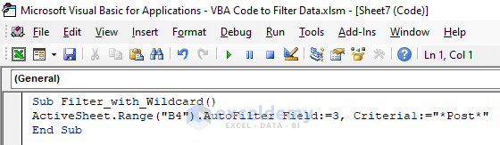
Sub Filter_with_Wildcard()
ActiveSheet.Range("B4").AutoFilter Field:=3, Criteria1:="*Post*"
End Sub- Minimize the VBA window.
Code Breakdown
- A Sub procedure, Filter_with_Wildcard() is created.
- Range(“B4”) is used to set the range.
- AutoFilter is used to Filter in Field:=3 means column 3.
- Criteria1:=”*Post*” is used to Filter the values containing ‘Post’.
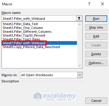
- Follow the third step in Example 1 to open the Macros dialog box.
- Select the Macro and click Run.
This is the output.
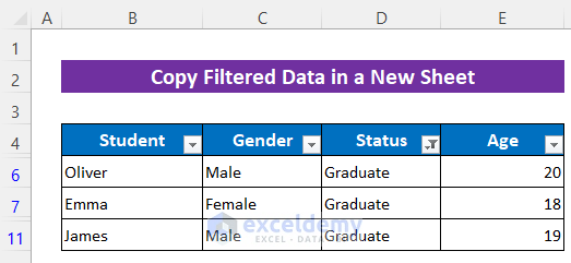
Example 7 – Copying Filtered Data in a New Sheet with Excel VBA
Steps:
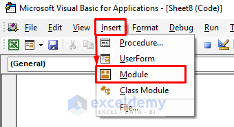
- Press Alt+F11 to open the VBA
- Click Insert > Module to open a module.
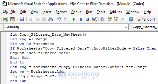
- Enter the following code.
Sub Copy_Filtered_Data_NewSheet()
Dim xRng As Range
Dim xWS As Worksheet
If Worksheets("Copy Filtered Data").AutoFilterMode = False Then
MsgBox "Noo filtered data"
Exit Sub
End If
Set xRng = Worksheets("Copy Filtered Data").AutoFilter.Range
Set xWS = Worksheets.Add
xRng.Copy Range("G4")
End Sub- Minimize the VBA
Code Breakdown
- A Sub procedure, Copy_Filtered_Data_NewSheet() is created.
- Two-variable- xRng is declared as Range and xWS as Worksheet.
- The IF statement checks the Filtered option.
- MsgBox shows the output.
- Worksheets(“Copy Filtered Data”).AutoFilter.Range selects the Filtered range and uses Add to add a new sheet.
- The Copy Range(“G4”) copies the Filtered data to the new sheet.
- Follow the third step in Example 1 to open the Macros dialog box.
- Select the Macro and click Run.
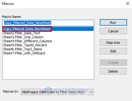
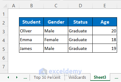
Excel opened a new sheet and copied the Filtered rows.
Read More: Excel VBA to Filter in Same Column by Multiple Criteria
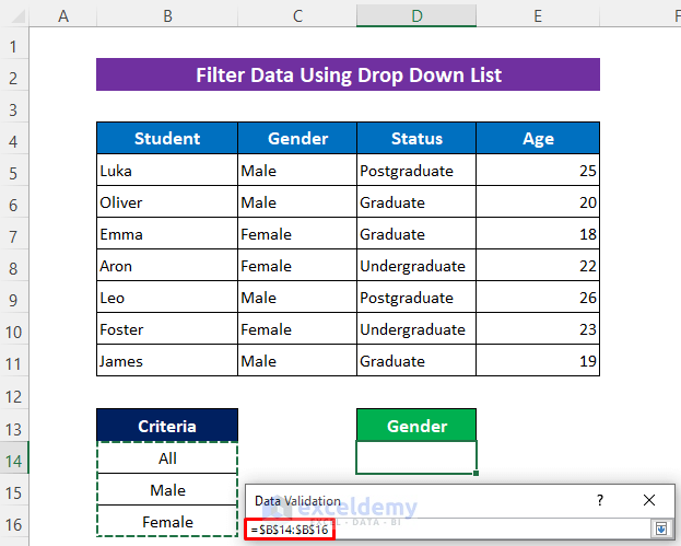
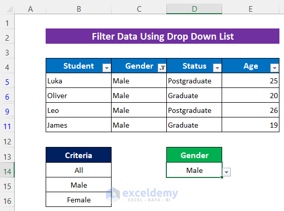
Example 8 – Applying a VBA Code to Filter Data Using a Drop-Down List
Steps:
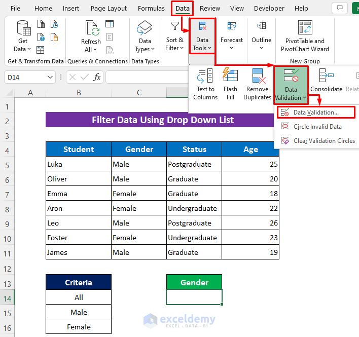
- Select D14.
- Click Data > Data Tools > Data Validation > Data Validation.
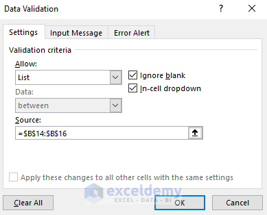
A dialog box will open.
- In the Allow drop-down menu, select List.
- In Source, clickOpen.
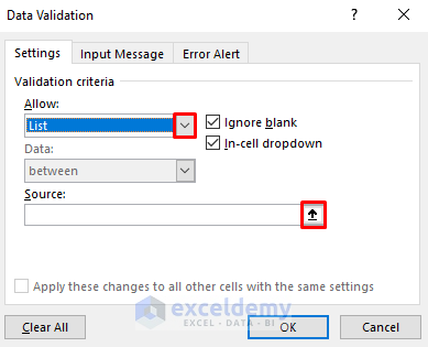
- Select the criteria range and press Enter.
- Click OK.
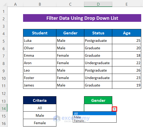
The drop-down list is displayed.
- Follow the two first steps in Example 1 to open the VBA window.
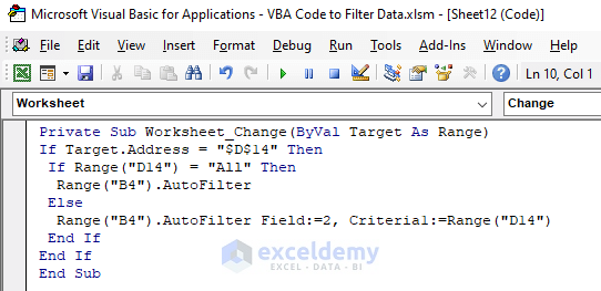
- Enter this code.
Private Sub Worksheet_Change(ByVal Target As Range)
If Target.Address = "$D$14" Then
 If Range("D14") = "All" Then
  Range("B4").AutoFilter
 Else
  Range("B4").AutoFilter Field:=2, Criteria1:=Range("D14")
 End If
End If
End Sub- Minimize the VBA window.
Code Breakdown
- A Private Sub procedure, Worksheet_Change(ByVal Target As Range) is created.
- Worksheet is selected from General and Change from Declarations.
- The Address is set to know the location.
- The IF statement used the AutoFilter method with Field and Criteria
Selected criteria from the drop-down list and the Filter will be activated.

This is the output after selecting Male.
Download Practice Workbook
Download the free Excel template here and practice.
Related Articles
- Excel VBA: Filter Based on Cell Value on Another Sheet
- Excel VBA: Filter Table Based on Cell Value
- Filter Different Column by Multiple Criteria in Excel VBA

