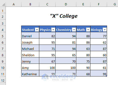
The following sample Table contains students’s marks.
Method-1 -Using a Structured Reference as an Excel Table Reference
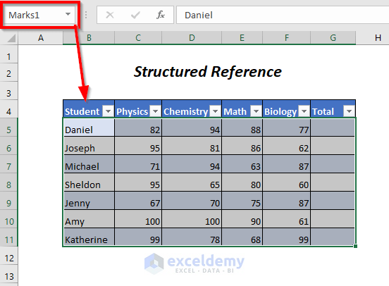
Marks1 is the sample table.
Steps:
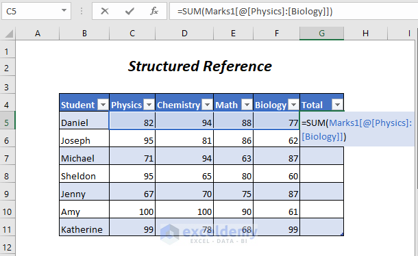
- Select G5 and enter the formula.
=SUM(C5:F5)C5:F5 is the range of the marks for Daniel and SUM adds these values.
By selecting the range C5:F5, Excel will convert them automatically to the structured reference system and modify the formula:
=SUM(Marks1[@[Physics]:[Biology]])Marks1 is the name of the Table, [Physics]:[Biology] is the range of the contiguous 4 columns; Physics, Chemistry, Math, and Biology. @ is the current row.
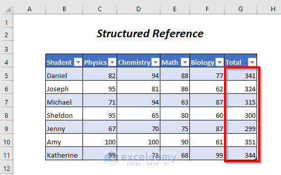
- Press ENTER, and the added marks for all rows will automatically be displayed in Total.
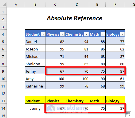
Method 2 – Using the Absolute Reference System as an Excel Table Reference
In Marks2 the SUMIF function will sum the marks of Physics, Chemistry, Math, and Biology for Jenny.
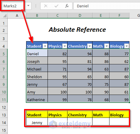
Steps:
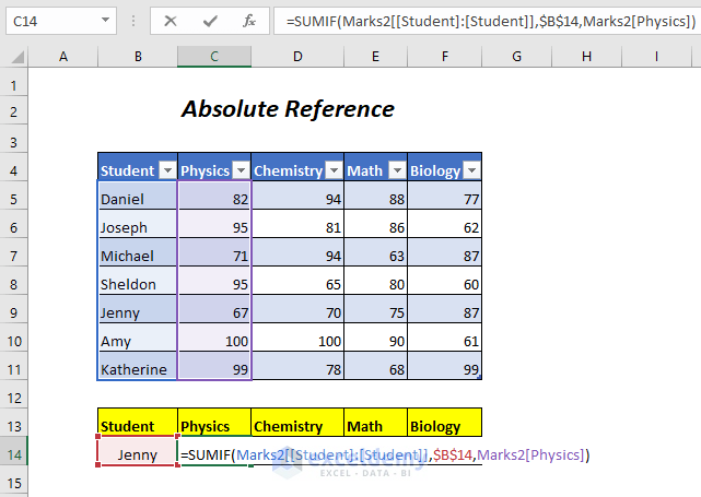
Enter the following formula in C14.
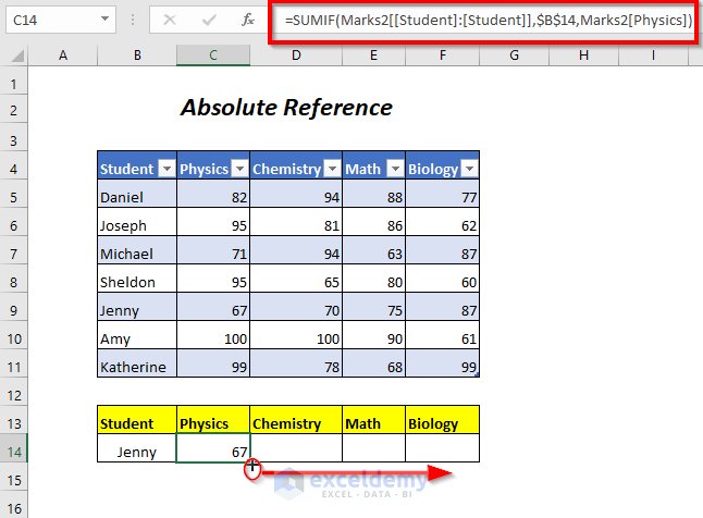
=SUMIF(Marks2[[Student]:[Student]],$B$14,Marks2[Physics])Marks2[[Student]:[Student]] is the range: Marks2 is the Table name and [Student]:[Student] is the absolute referencing in the Student column; $B$14 is the criteria, and Marks2[Physics] is the sum range: the Physics column.
- Press ENTER and drag the Fill Handle tool to the right.
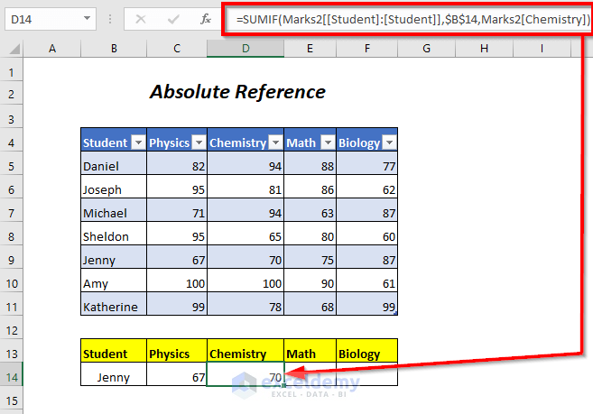
It will copy the formula to cell D14 and showcase the following formula
=SUMIF(Marks2[[Student]:[Student]],$B$14,Marks2[Chemistry])The absolute referenced data range is not changed, only Marks2[Physics] changed to Marks2[Chemistry] to return the Chemistry.
- Copy the formula for Math and Biology to see the marks for Jenny.
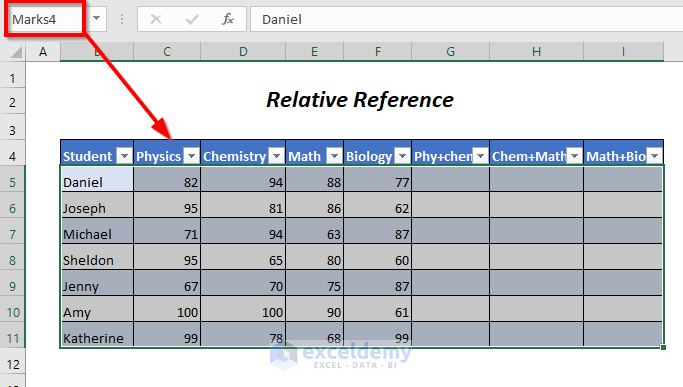
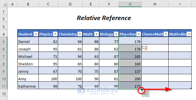
Method 3- Using the Relative Reference System as an Excel Table Reference
In table Marks3, marks in Physics and Chemistry, Chemistry and Math, Math and Biology will be summed for the students in the Phy+chem, Chem+Math, and Math+Bio columns.
Steps:
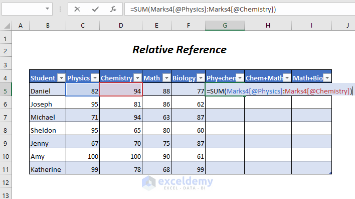
- Enter the following formula in G5
=SUM([Marks4[@Physics]:[Marks4[@Chemistry])Marks4 is the Table name, [@Physics] and [@Chemistry] is the corresponding row in the Physics and Chemistry column.
The relative reference system is Marks4[@Physics]:[Marks4[@Chemistry]
- Press ENTER to see the sum of marks in the Physics and Chemistry columns. Excel will change the formula into:
=SUM([@Physics]:[@Chemistry])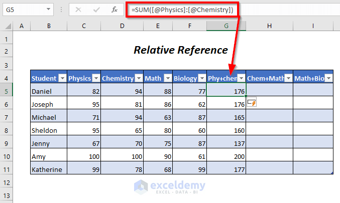
- Select the cells in the Phy+chem column and drag the Fill Handle tool to the right.
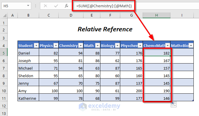
- In the Chem+Math column, the formula is the following:
=SUM([@Chemistry]:[@Math])It will sum up the marks of Chemistry and Math for each student.
The sum of Math and Biology marks is displayed in the Math+Bio column.
=SUM([@Math]:[@Biology])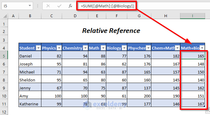
Method 4- Referencing Multiple Non-Contiguous Columns Using an Excel Table Reference
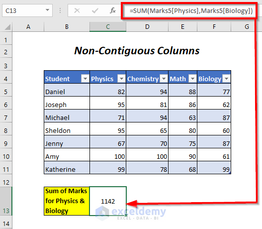
Here, Marks5 is the Table name. Marks in Physics and Biology will be added.
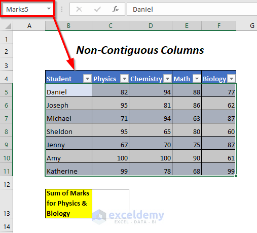
Steps:
- Enter the following formula in C13
=SUM(Marks5[Physics],Marks5[Biology])Marks5 is the Table name and [Physics], [Biology] are the Physics and Biology columns.
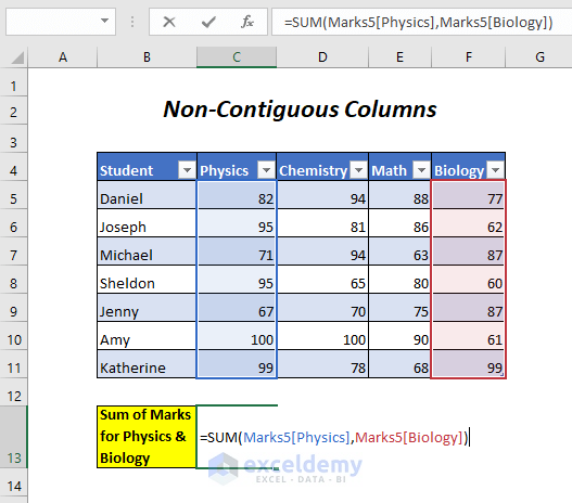
- Press ENTER to see the sum of the marks for all students in Physics and Biology.
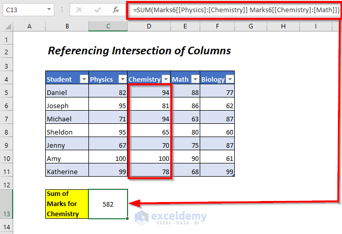
Method 5 – Referencing the Intersection of Columns Using an Excel Table Reference
Here, Marks6 is the Table name. Marks in Chemistry will be added for all students.
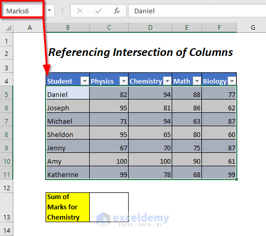
Steps:
- Enter the following formula in C13.
=SUM(Marks6[[Physics]:[Chemistry]] Marks6[[Chemistry]:[Math]])Marks6 is the Table name and [Physics]:[Chemistry] and [Chemistry]:[Math] are the two ranges. The intersected column is [Chemistry] which will be referenced.
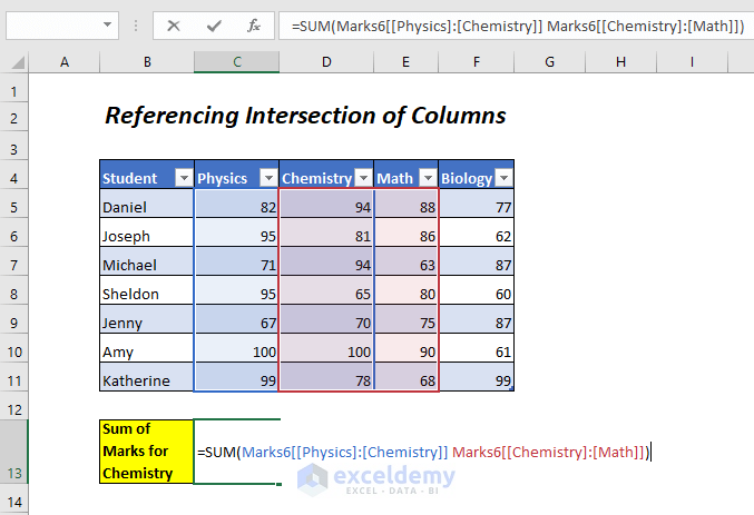
- Press ENTER to see the sum of marks for all students in Chemistry.
Similar Readings
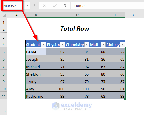
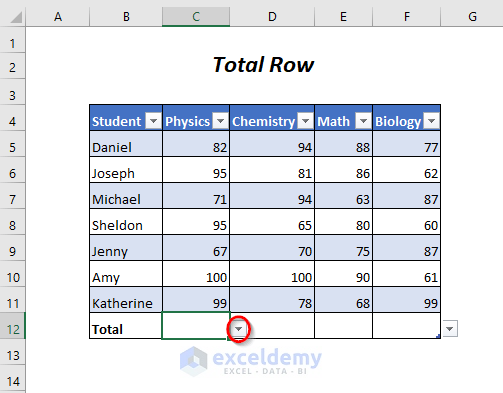
Method 6 – Using the Total Row Option for Filtered Tables
In Marks7 the Total Row option will be used to sum the marks.
Steps:
- Select any cell in the Table.
- Go to the Table Design Tab >> Table Style Options >> click Total Row.
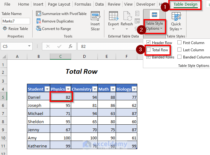
A new row (Total) will be added.
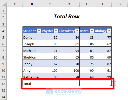
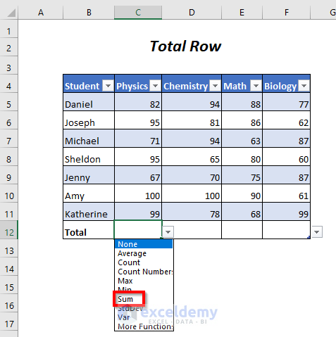
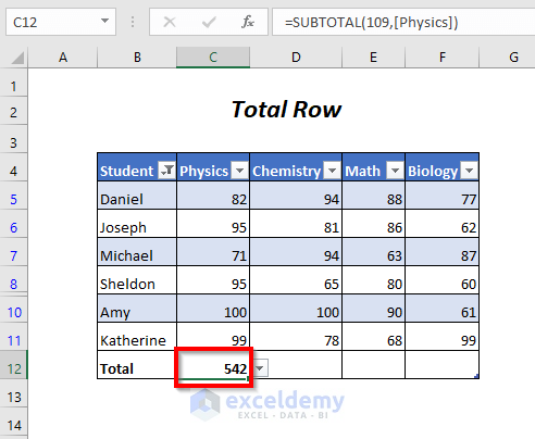
- Click C12 and click the dropdown sign.
- Select Sum.
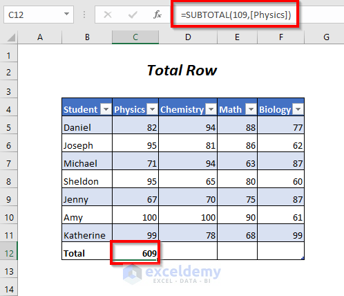
You will see the sum of the marks in Physics and the following formula will be displayed.
=SUBTOTAL(109,[Physics])SUBTOTAL will add up the visible values of the filtered table, 109 is for SUM, and [Physics] is the column name.
- Hide the marks of a student (Jenny, here) by unclicking her name and clicking OK.
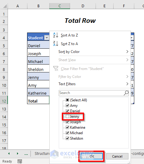
The total marks in Physics are changed to 542 as SUBTOTAL only works for visible cells.
- Unhide Jenny and see the sum of the marks in Chemistry, Math, and Biology.
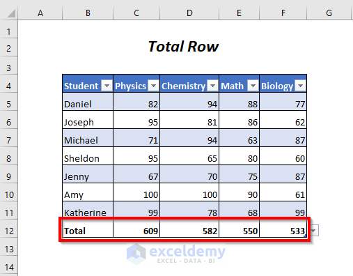
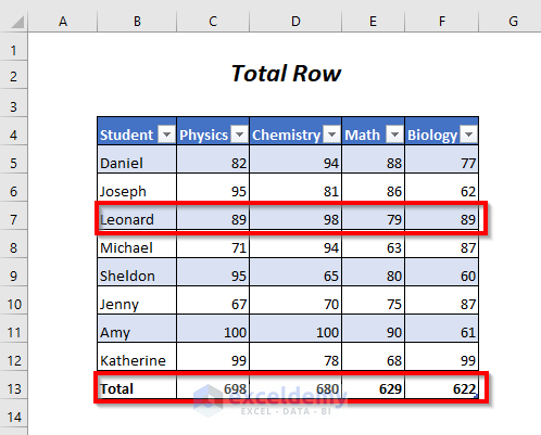
- Adding new data (Leonard’s marks) will update Total values.
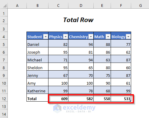
- Deleting Leonard’s data returns the previous results.
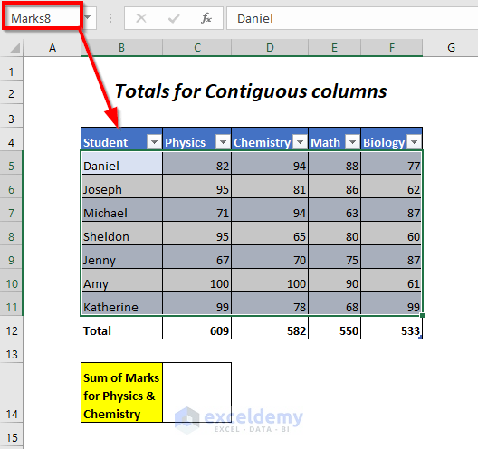
Method 7 – Referencing the Totals for Multiple Contiguous Columns Using an Excel Table Reference
In Marks8 the reference of the totals will be used and the total value of the marks in Physics and Chemistry will be summed.
Steps:
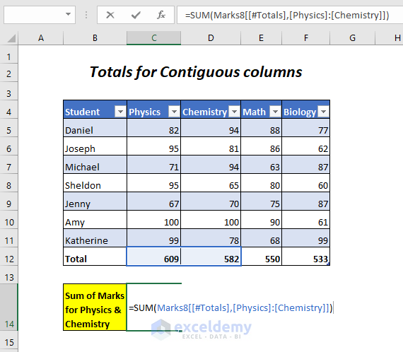
- Enter the following formula in C14
=SUM(Marks8[[#Totals],[Physics]:[Chemistry]])Marks8 is the Table name, [#Totals] is the Total row, [Physics]:[Chemistry] is the range in the Physics and Chemistry column.
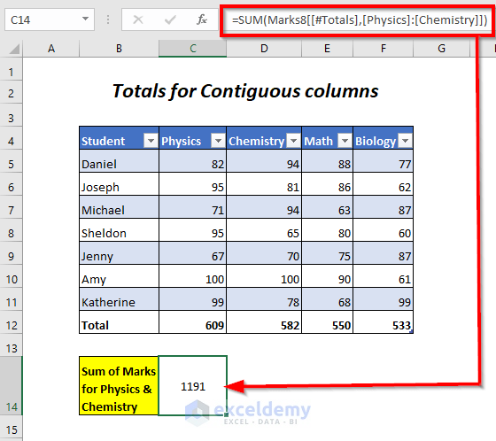
- Press ENTER to see the sum of marks in Physics and Chemistry.
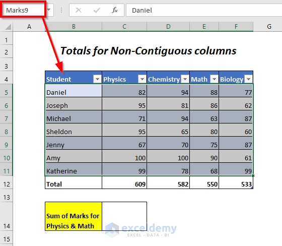
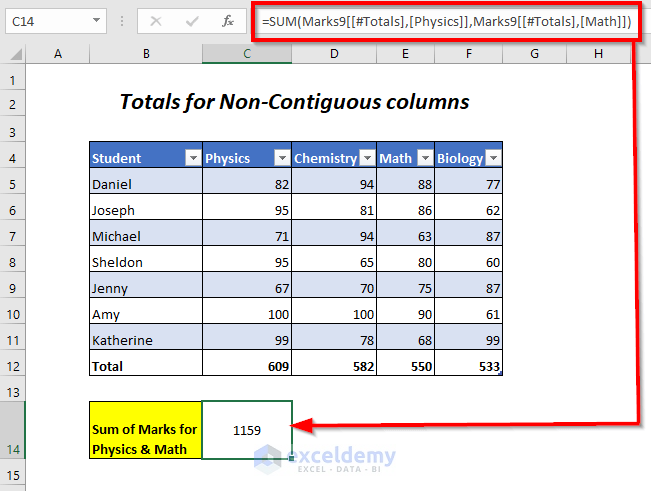
Method 8 – Referencing the Totals for Multiple Non-Contiguous Columns Using an Excel Table Reference
In Marks9 the reference of the totals will be used and the total value of the marks in Physics and Math will be summed.
Steps:
- Enter the following formula in C14.
=SUM(Marks9[[#Totals],[Physics]],Marks9[[#Totals],[Math]])Marks9 is the Table name, [#Totals] is the Total row, [Physics], and [Math] are the Physics and Math columns.
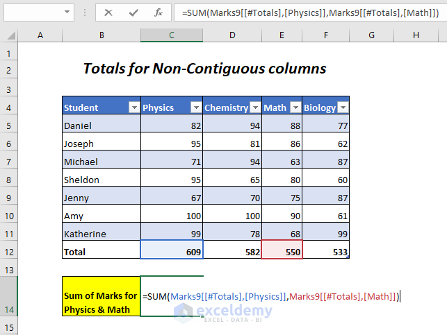
- Press ENTER.
You will see the sum of the marks for the two non-contiguous columns Physics and Math.
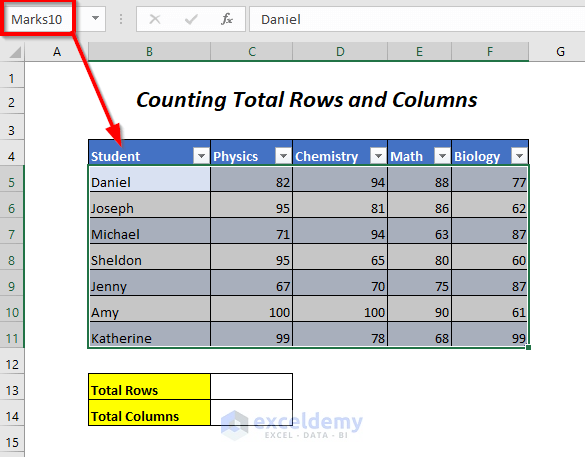
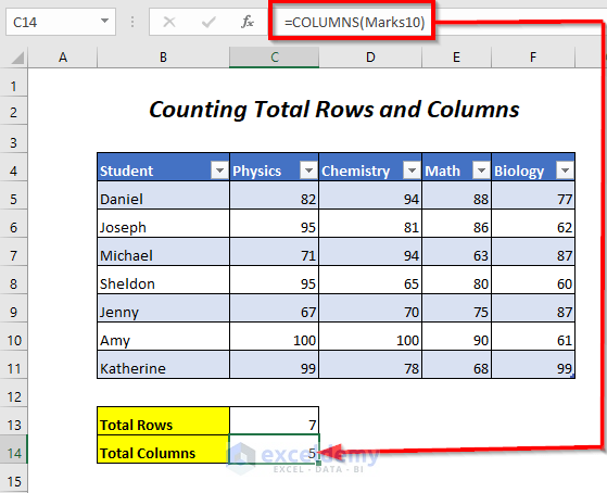
Method 9 – Counting Total Rows and Columns Using an Excel Table Reference
Total rows and columns in Marks10 will be counted by using the ROWS and COLUMNS functions.
Steps:
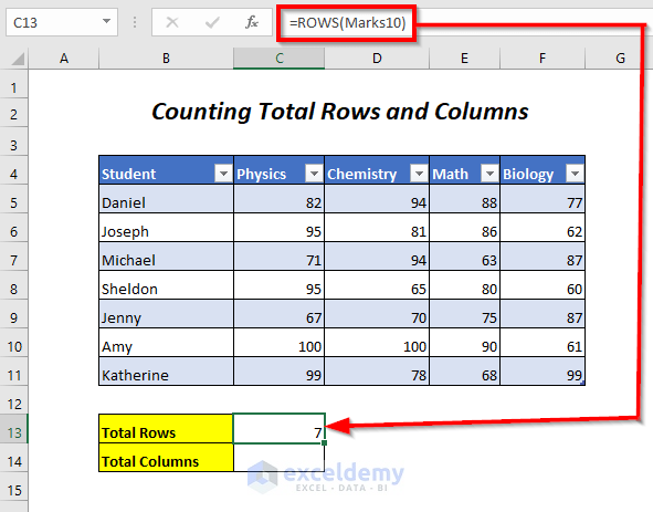
- Enter the following formula in C13
=ROWS(Marks10)ROWS will determine the number of rows in Marks10.
- Use the following formula in C14
=COLUMNS(Marks10)COLUMNS will return the total number of columns in Marks10.
This is the output.
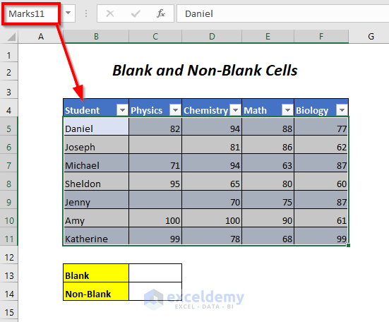
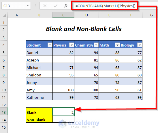
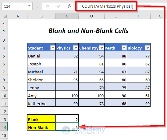
Method 10 – Counting Blank and Non-Blank Cells Using an Excel Table Reference
The COUNTBLANK function and the COUNTA function will return the total blank and non-blank cells in the Physics column, in Marks11.
Steps:
- Enter the following formula in C13.
=COUNTBLANK(Marks11[Physics])COUNTBLANK will determine the number of blank cells in the Physics column.
- Use the following formula in C14
=COUNTA(Marks11[Physics])COUNTA will determine the number of non-blank cells in the Physics column.
This is the output.
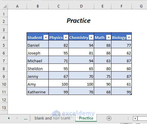
Practice Section
Practice here.
Things to Remember
- Structured references in Excel are tied to specific rows, so when you sort a table, the reference points to the same row but may now refer to a different value.
- To maintain a reference to the same cell after sorting, consider using functions like INDEX-MATCH or XLOOKUP, which dynamically locate and return values even after sorting changes the order of rows.
Download Workbook
Structured Reference Excel: Knowledge Hub
- Applications of Absolute Structured References with Table Formulas
- Use HLOOKUP with Structured Reference
- Lock a Structured Reference
- Reference a Dynamic Component of a Structured Reference
- What is an Unqualified Structured Reference
- Use IF Function and Structured Reference
<< Go Back to Table Formula | Excel Table | Learn Excel
Get FREE Advanced Excel Exercises with Solutions!

somewhere you should tells us a table reference can only be on the same row – or tell us how to reference the same cell after a sort has changed the row order.
Hello Chad Sellers,
Thank you for your feedback! You’re correct that structured table references typically apply to the same row, which can cause confusion after sorting changes the row order. I’ve updated the article to include a section that addresses how structured references behave after sorting and how to maintain consistent references to the same cell even when the row order changes.. You can use INDEX-MATCH combination or the XLOOKUP function to maintain references correctly after sorting. Your input is greatly appreciated!
Regards
ExcelDemy
It appears to me you have a typo near the beginning:
=SUM(C5:C7)
C5:C7 is the range of the marks for Daniel and SUM adds these values.
By selecting the range C5:C7, Excel will convert them automatically to the structured reference system and modify the formula:
=SUM(Marks1[@[Physics]:[Biology]])
Shouldn’t it be “=SUM(C5:F5)” to sum the marks row for Daniel and match the next “=SUM(Ma…” statement. C5:C7 would be the marks of 3 names for Physics only (Daniel, Joseph and Michael).
Hello Chad Sellers,
Thank you for your feedback! You’re absolutely right—thank you for catching that! The correct range to sum Daniel’s marks should indeed be =SUM(C5:F5), which sums the marks across all subjects for Daniel. I’ve updated the article to reflect this change, ensuring it matches the subsequent structured reference example. I appreciate your attention to detail and for bringing this to my attention!
Regards
ExcelDemy