We will show you four distinct formulas to remove the last 3 characters in Excel with ease. We’ll use a simple dataset that contains employee information. All the names have the last name “Roy” which we’ll delete.
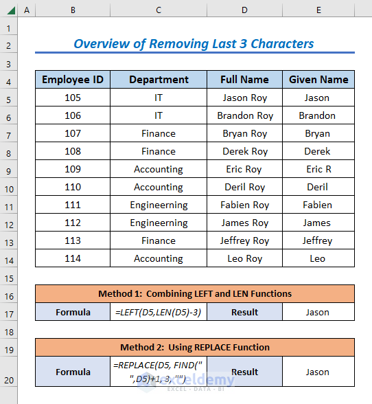
How to Remove the Last 3 Characters in Excel: 4 Easy Ways
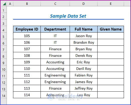
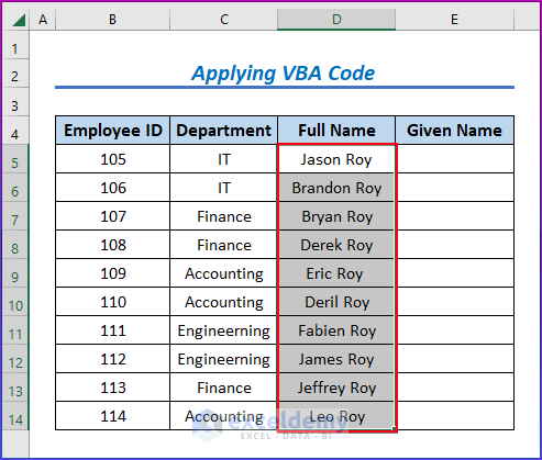
Here’s the starting dataset we’ll use. We’ll focus on the Full Name column to remove the last three characters from the cells in it.
Method 1 – Combining LEFT and LEN Functions to Remove the Last 3 Characters in Excel
Steps:
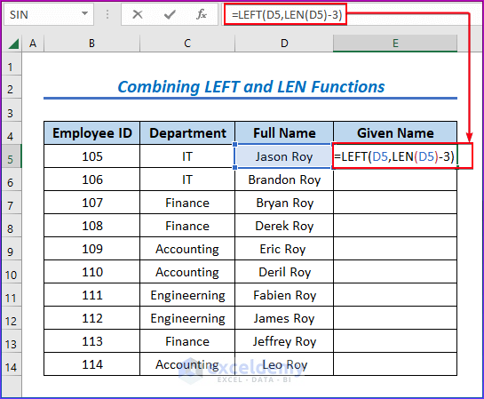
- Select the cell E5.
- Insert this formula.
=LEFT(D5,LEN(D5)-3)
- Press the Enter button.
- LEN(D5)-3 ▶ calculates the length of the text, “Jason Roy” and then subtracts the result with 3.
- D5 ▶ refers to the cell address of the text “Jason Roy”.
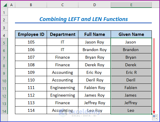
- =LEFT(D5,LEN(D5)-3) ▶ truncates the last 3 characters i.e. “Roy” from the text “Jason Roy”.
- Drag the Fill Handle icon to the end of the Given Name column.
Read more: How to Remove Last Character in Excel
Method 2 – Using the REPLACE Function to Delete the Last 3 Characters in Excel
Steps:
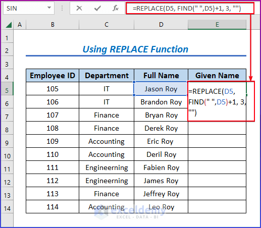
- Select cell E5.
- Insert the following formula.
=REPLACE(D5, FIND(" ",D5)+1, 3, "")
- Hit Enter.
- “” ▶ refers to a null string in Excel.
- 3 ▶ refers to the last 3 characters in a text line.
- FIND(” “,D5)+1 ▶ finds the starting number of the last 3
- ” “ ▶ used for the detection of the end of a text line.
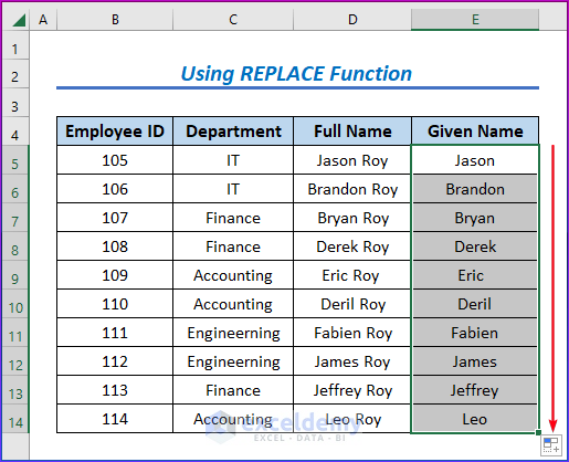
- =REPLACE(D5, FIND(” “,D5)+1, 3, “”) ▶ truncates the last 3 characters i.e. “Roy” from the text “Jason Roy”.
- Drag the Fill Handle icon to the end of the Given Name column.
Method 3 – Using the Flash Fill Feature to Remove the Last 3 Characters in Excel
Steps:
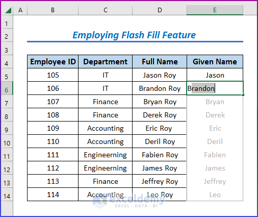
- Select cell E5 and type Jason in it (since that’s the value in the adjacent cell).
- Press Enter.
- In the next cell, E6, start typing Brandon.
- Excel has already figured out the pattern and suggests a preview for all the following names.
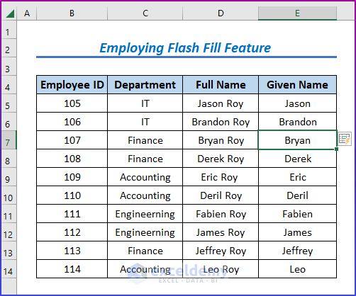
- Press the Enter button again.
- You may need to insert the second name manually to get the right pattern.
- Excel autocompletes the Given Name column.
Read more: How to Remove First 3 Characters in Excel
Method 4 – Applying VBA Code to Remove the Last 3 Characters in Excel
Steps:
- Select the range (D5:D14).
- Press Alt + F11 keys to open the VBA window.
- Go to Insert and select Module.

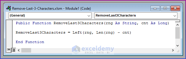
- Copy the following VBA code:
Public Function RemoveLast3Characters(rng As String, cnt As Long)
RemoveLast3Characters = Left(rng, Len(rng) - cnt)
End Function- Press Ctrl + V to paste the above VBA code into the module.
- Save the VBA code and go back to your spreadsheet.
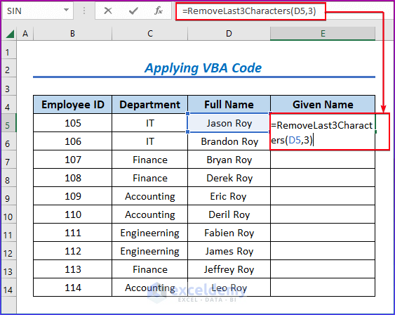
- Select cell E5.
- Insert this formula.
=RemoveLast3Characters(D5,3)
- Press Enter.
- Drag the Fill Handle icon to the end of the Given Name column.
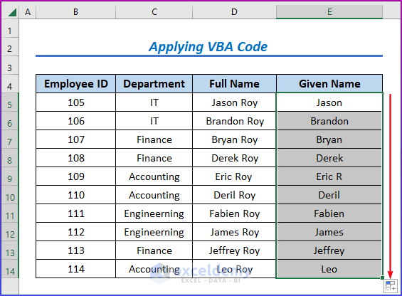
The function =RemoveLast3Characters(Text,Number)is a user-defined function. You can use this function along with the VBA code to delete any number of last characters from a string. Just input any desired number into the Number slot of the function.
Things to Remember
Be careful about the syntax of the functions.
Insert the data ranges carefully into the formulas.
(“”) refers NULL String in Excel.
Read More: How to Remove Last Character from String Using VBA in Excel
Related Articles
- How to Remove First Character in Excel
- How to Remove Last Digit in Excel
- How to Remove the First Character from a String in Excel with VBA
<< Go Back To Excel Remove Characters from Right | Excel Remove Characters | Data Cleaning in Excel | Learn Excel
Get FREE Advanced Excel Exercises with Solutions!
