How to Remove Last Digit in Excel (6 Quick Methods)

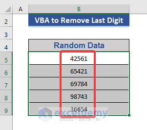
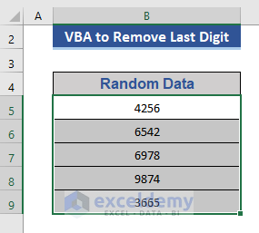
Let’s use the following dataset of some random data to explain how to remove last digits.

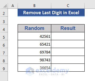
How to Remove Last Digit in Excel: 6 Quick Methods

Method 1 – Use TRUNC Function to Remove Last Digit

Syntax:

Steps:

• Go to cell C5.
• Write the below formula:

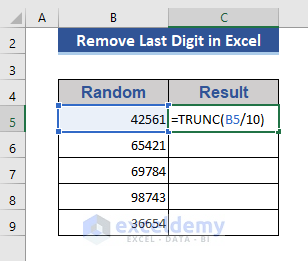
• Press the Enter key.

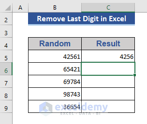
We can see that the last digit is removed from the data of cell B5.

• Drag the Fill Handle icon towards the last cell.

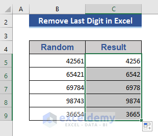
We divided all the values by “10” and removed all the fractional values with TRUNC.

Read More: How to Remove Last Character in Excel

Method 2 – Insert LEFT Function with LEN Function to Remove Last Digit.

Steps:

• Go to cell C5.
• Write the following formula in that cell:

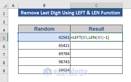
• Press Enter.

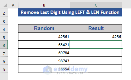
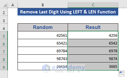
• Drag the Fill handle icon to the last cell.

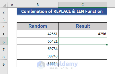
Method 3 – Combine REPLACE & LEN Functions to Remove Last Digit

The REPLACE function replaces several digits or characters from a series based on your choice.

Steps:

• Put the following formula in cell C5:

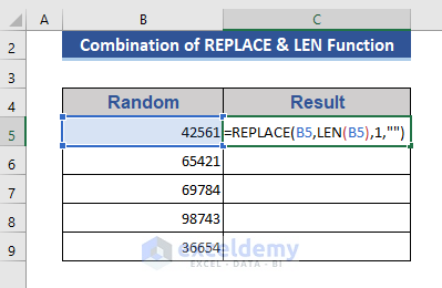
• Hit Enter.

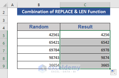
• Drag the Fill Handle icon towards the last cell.

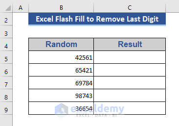
Method 4 – Remove Last Number Using Excel Flash Fill

This is our dataset. We want to remove the last digit from this dataset.

Steps:

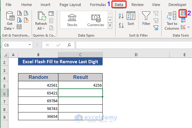
• Manually input the first result into cell C5.

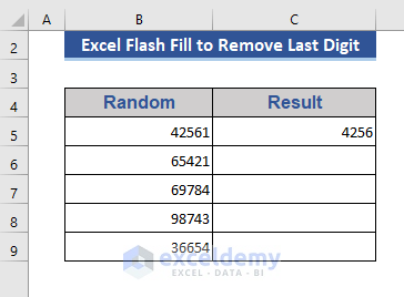
• Click on cell C6.
• Go to the Data tab.
• Select the Flash Fill option.

• After selecting the Flash Fill our data becomes the below image.

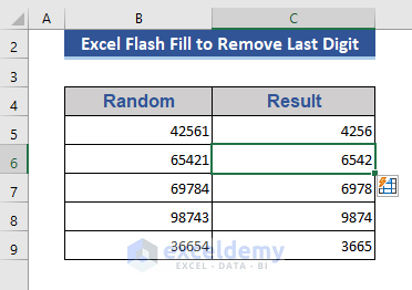
You can also use Ctrl + E to shortcut to Flash Fill for a selection.

Note:

If Flash Fill is turned off, then turn on this in the following way.

• Go to File and select Options.
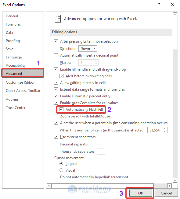
• Select the Advanced tab.
• Tick Automatically Flash Fill.
• Press OK.

Read More: How to Remove First Character in Excel

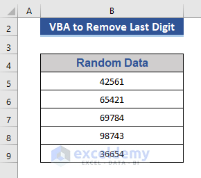
Method 5 – VBA Macro Code to Remove Last Digit in Excel

The code will replace the values inside cells with new ones.

Steps:

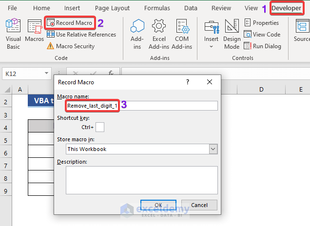
• Go to the Developer tab.
• Click on Record Macro.
• Put Remove_last_digit_1 on the Macro name box.
• Click on OK.

• Click on Macros and select Remove_last_digit_1 from the Macro dialog box.
• Press the Step Into.

• Copy this code in the command window and save:

Sub Remove_last_digit_1()
Dim last As Range
For Each last In Selection
If (Not last.HasFormula) And (Application.WorksheetFunction.IsNumber(last)) Then
last = Left(last, Len(last) - 1)
End If
Next last
End Sub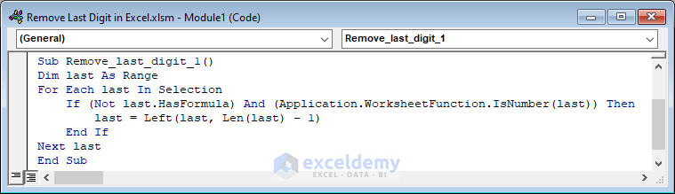

• Select the data from the Excel worksheet.

• Press the play button in the VBA main tab to run the code or use F5.

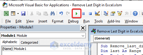
• This is our final result.

Read More: How to Remove Last Character from String Using VBA in Excel

Method 6 – Build a VBA Function to Remove Last Digit

Steps:

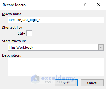
• Create a new macro named Remove_last_digit_2.
• Press OK.

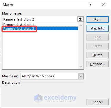
• Step Into the Remove_last_digit_2 macro following way shown in the previous method. Or, press Alt+F8.

• Copy the following code in the command window:

Function RemoveLastDigit(input1 As String, num_digit As Long)
RemoveLastDigit = Left(input1, Len(input1) - num_digit)
End Function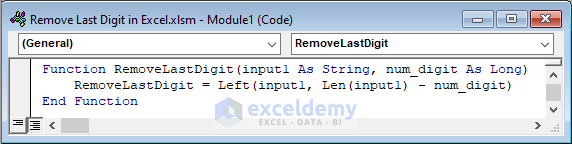

• Save the code and go to the Excel worksheet.
• Write this formula into C5:

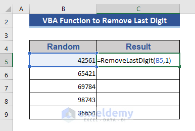
• Press Enter.

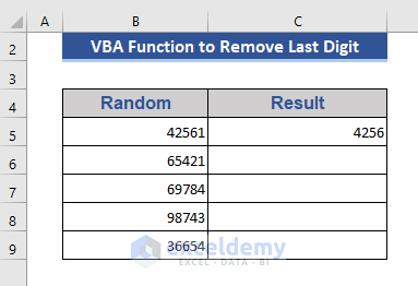
• Drag the Fill Handle icon to get the values of the rest of the cells.

This is a customized function. We used “1” in the last argument to remove only the last digit. To remove more than one digit, change this argument as needed.

Read More: How to Remove the First Character from a String in Excel with VBA

Things to Remember

• The TRUNC function works only with numeric values.
• When applying the LEN function with other functions, you must subtract “1” as mentioned in the formula.

Download Practice Workbook

Related Articles

• How to Remove the Last 3 Characters in Excel
• How to Remove First 3 Characters in Excel

<< Go Back To Excel Remove Characters from Right | Excel Remove Characters | Data Cleaning in Excel | Learn Excel