Permutation tables are very useful when the order and position of our data are important. In computer science, they play an essential role in sorting data or algorithms; in biology, they are used to describe the RNA and DNA sequences of a genome; and in quantum physics, they are used for representing the different possible states of a certain particle.
We’ll cover 4 different methods to create a Permutation Table in Excel in this tutorial.
Method 1 – Using Combined Excel Functions to Determine Permutation Table
For this method we’ll use a combination of the INDEX, INT, ROW, and COUNTA functions to determine all permutations of some data.
The reference form of the INDEX function returns a value (or values) from multiple ranges. The INT function returns the nearest integer of a decimal number. The ROW function returns the row number for a given reference. And the COUNTA function is generally used to count the cells containing non-empty character(s) only.
Steps:
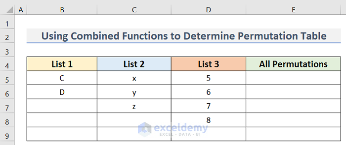
- Create a dataset similar to the below image. where we have the List 1 dataset in Column B, the List 2 dataset in Column C, and List 3 dataset in Column D. The All Permutations that we determine will be shown in Column E.
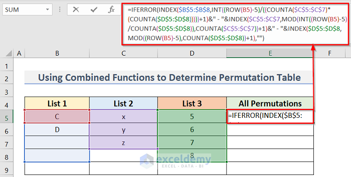
- Enter the following formula in cell E5:
=IFERROR(INDEX($B$5:$B$8,INT((ROW(B5)-5)/((COUNTA($C$5:$C$7)*(COUNTA($D$5:$D$8)))))+1)&" - "&INDEX($C$5:$C$7,MOD(INT((ROW(B5)-5)/COUNTA($D$5:$D$8)),COUNTA($C$5:$C$7))+1)&" - "&INDEX($D$5:$D$8,MOD((ROW(B5)-5),COUNTA($D$5:$D$8))+1),"")
How Does the Formula Work?
- COUNTA($D$5:$D$8) —-> calculates the number of items (non empty cells) in the range D5:D8.
- Output: 4
- ROW(B5)-5 —-> returns the number argument for the MOD function.
- Output: 0
- MOD((ROW(B5)-5),COUNTA($D$5:$D$8))+1 —-> turns into
- MOD({0},4)+1 —-> which returns
- Output: {1}
- INDEX($D$5:$D$8,MOD((ROW(B5)-5),COUNTA($D$5:$D$8))+1) —-> simplifies to
- INDEX($D$5:$D$8,{1}) —-> which results in the value of cell D5.
- Output: 5
- INDEX($C$5:$C$7,MOD(INT((ROW(B5)-5)/COUNTA($D$5:$D$8)),COUNTA($C$5:$C$7))+1) —-> similarly returns the cell value of C5.
- Output: x
- INDEX($B$5:$B$8,INT((ROW(B5)-5)/((COUNTA($C$5:$C$7)*(COUNTA($D$5:$D$8)))))+1) —-> follows similar calculations and returns the List 1 value from B5.
- Output: C
- Finally, the whole formula simplifies to
- IFERROR(“C – x – 5″,””) —-> which returns
- Output: C -x – 5
Here, we are making a permutation table where List 3 items will appear with each item in List 2. Then they will combine with each item in List 1. So the output will be C – x – 5, C – x – 6, and so on. As List 1, List 2, and List 3 have 2, 3, and 4 items respectively, the number of possible permutations will be 2 x 3 x 4 or 24.
- Use the Fill Handle to apply the formula to the cells below.
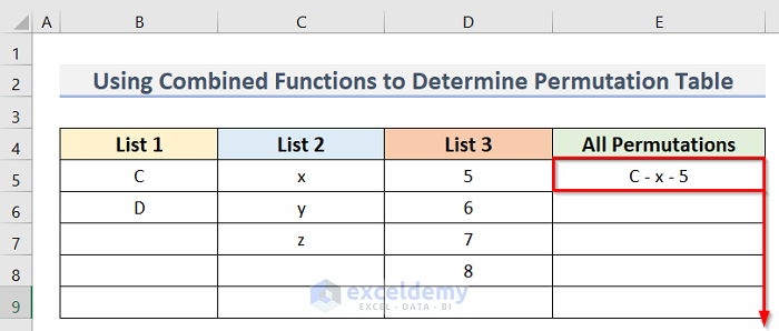
- Press Enter to return the final result.
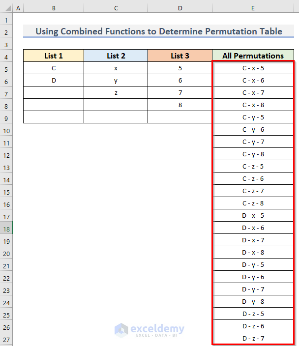
A table of all possible permutations is created.
Read More: How to Generate or List All Possible Permutations in Excel
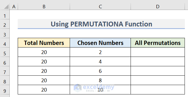
Method 2 – Using the PERMUTATIONA Function to Create Permutation Table
The PERMUTATIONA function can determine all the possible permutations in Excel.
- Create a dataset like in the below image, where we have the Total Numbers dataset in Column B and the Chosen Numbers dataset in Column C. The All Permutations that we determine will go in Column D.
- Enter the following formula in cell D5:
=PERMUTATIONA(B5,C5)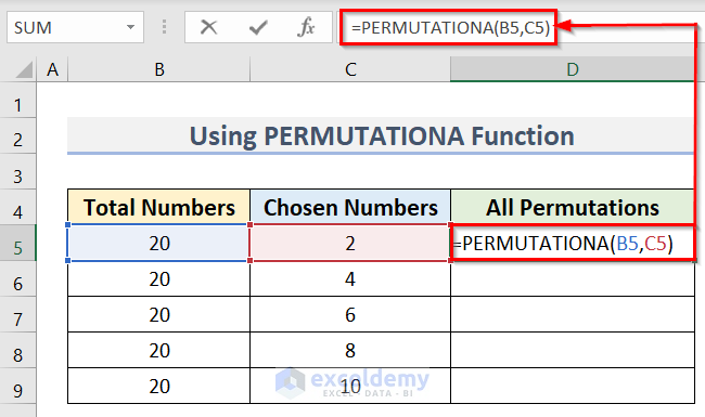
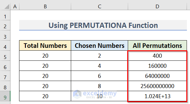
- Use the Fill Handle to apply the formula to the cells below.
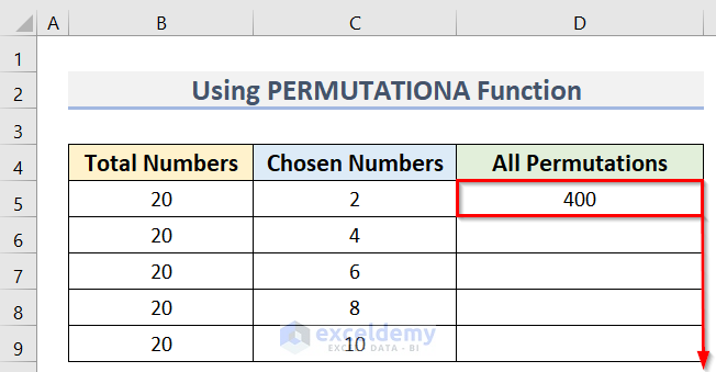
Our Permutation table is returned.
Method 3 – Using the PERMUT Function
The PERMUT function works the same as the PERMUTATIONA function with a slight change. In cases where you need to count the repetitions, use the PERMUTATIONA function, but if you don’t need to count the repetitive values, you can instead use the PERMUT function.
Steps:
- Arrange a dataset similar to Method 2.
- Enter the following formula in cell D5:
=PERMUT(B5,C5)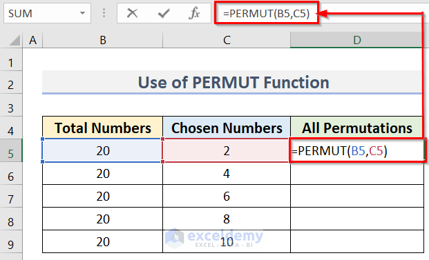
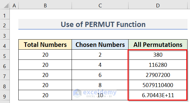
- Use the Fill Handle to apply the formula to the cells below.

The final result using the PERMUT function is returned.
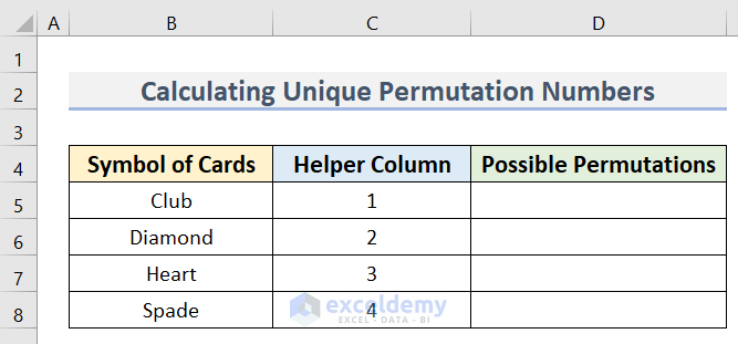
Method 4 – Calculating Unique Permutation Numbers
We can determine only the unique permutations by using a combination of the COUNTA and PERMUT functions. The PERMUT function determines the permutation with a count of no repetitive values and the COUNTA function counts the total number of the values and represents them.
Steps:
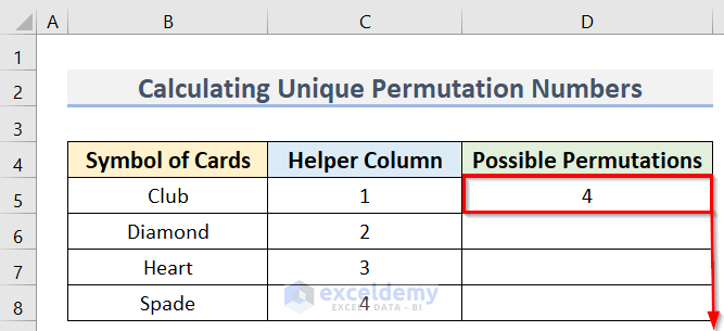
- Arrange a dataset similar to the below image. We have the Symbol of Cards dataset in Column B and the Helper Column in Column C. We will determine Possible Permutations in Column D.
- Enter the following formula in cell D5:
=PERMUT(COUNTA($B$5:$B$8),C5)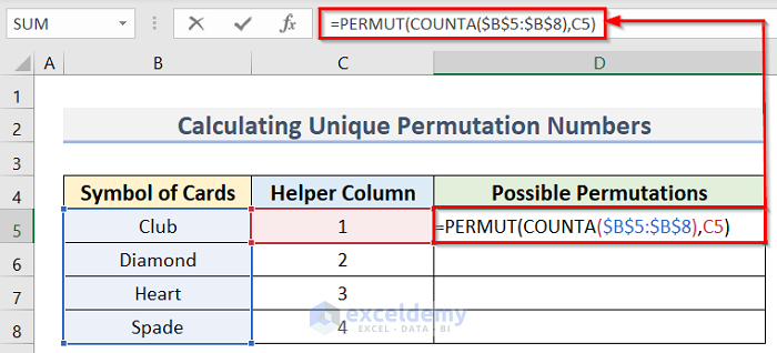
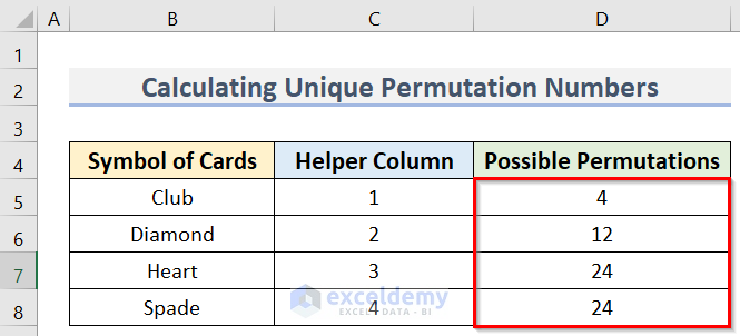
- Use the Fill Handle to apply the formula to the cells below.
The final result of only unique permutations is returned.
Note:
As we have 4 data points, the number we use in the Helper Column cannot exceed 4. The numbers must be Natural Numbers.
How to Use Combined Functions to Determine Combination in Excel
We can determine Combinations by combining the functions INDIRECT, ROW, COUNTA, TEXTJOIN, and TRIM.
The ROW function returns the row number for a given reference. The COUNTA function is generally used to count the cells containing non-empty character(s) only. The INDIRECT function is generally applied to store a cell reference and then use the reference value with other functions to perform multiple operations. The TEXTJOIN function concatenates a list or range of text strings into a single string using a delimiter, and can include both empty and non-empty cells. The TRIM function removes extra spaces from a text string.
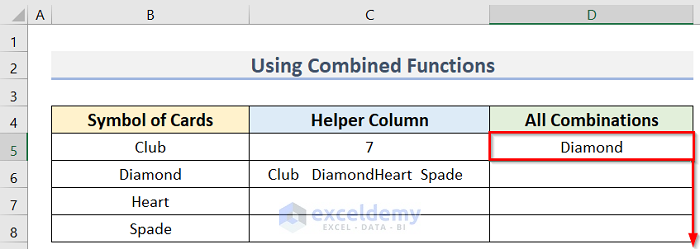
Using these combined functions, let’s determine the possible combinations, first for a Diamond card and then for a Club.
Steps:
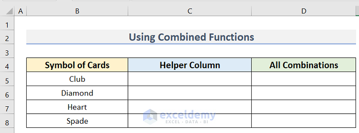
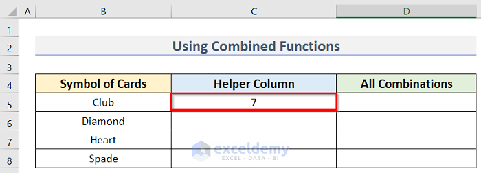
- Arrange a dataset similar to the below image. We have the Symbol of Cards dataset in Column B and the Helper Column in Column C. We will determine All Combinations in Column D.
- Enter the following formula in cell D5:
=MAX(LEN(B5:B8))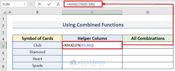
- Press Enter to return the result for this cell.
- Enter the following formula in cell D5:
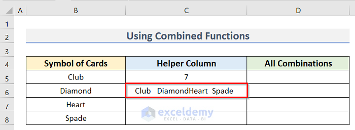
=CONCAT(B5:B8&REPT(" ",C5-LEN(B5:B8)))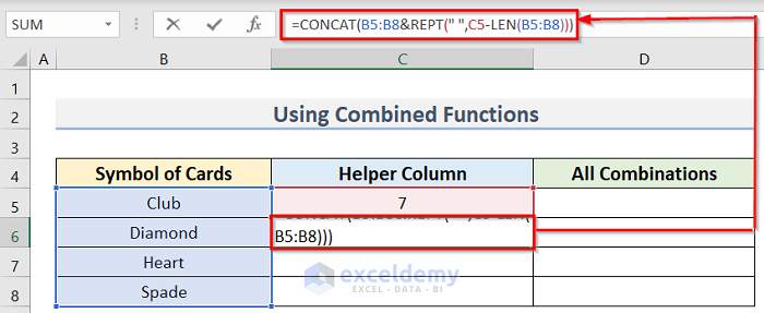
- Press Enter to return the result for this cell.
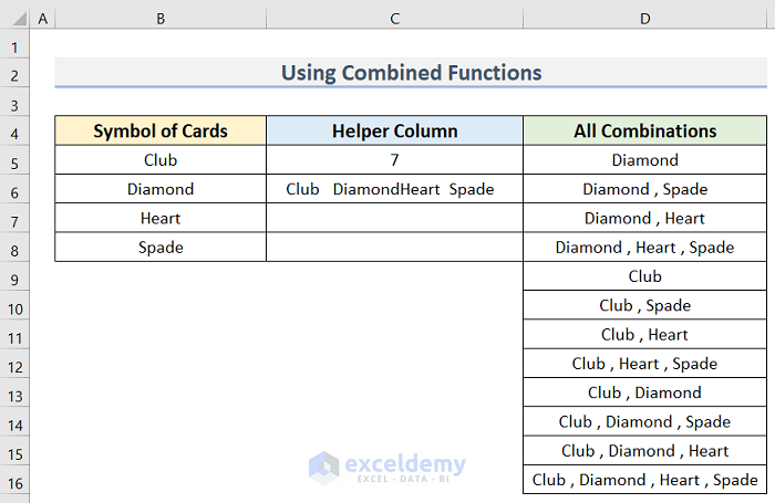
- Enter the following formula in cell D5:
=IF(ROW()>2^(COUNTA($B$5:$B$8)),"",TEXTJOIN(" , ",TRUE,IF(MID(TEXT(DEC2BIN(ROW()-1),REPT("0",COUNTA($B$5:$B$8))),ROW(INDIRECT("1:"&COUNTA($B$5:$B$8))),1)+0,TRIM(MID($C$6,(ROW(INDIRECT("1:"&COUNTA($B$5:$B$8)))-1)*$C$5+1,$C$5)),"")))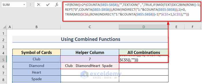
How Does the Formula Work?
- COUNTA($B$5:$B$8): the value range we want to count.
- ROW(INDIRECT(“1:”&COUNTA($B$5:$B$8)))-1)*$C$5+1,$C$5)): we use the INDIRECT function to mark it for many applications. The ROW function sets it as the row input value.
- IF(ROW()>2^(COUNTA($B$5:$B$8)): the condition we want to use.
- TRIM(MID($C$6,(ROW(INDIRECT(“1:”&COUNTA($B$5:$B$8)))-1)*$C$5+1,$C$5)): the TRIM function removes extra space and the MID function works on the middle column of our data.
- IF(ROW()>2^(COUNTA($B$5:$B$8)),””, TEXTJOIN(“, “, TRUE, IF(MID(TEXT(DEC2BIN(ROW()-1), REPT(“0”, COUNTA($B$5:$B$8))), ROW(INDIRECT(“1:”&COUNTA($B$5:$B$8))),1)+0, TRIM(MID($C$6,(ROW(INDIRECT(“1:”&COUNTA($B$5:$B$8)))-1)*$C$5+1,$C$5)),””))): the combination of all the sections along with the TEXTJOIN function. The whole formula combines all the functions to show all combinations in our dataset.
- Press Enter.
- Use the Fill Handle to apply the formula to the cells below.
- Press Enter to see the final result.
How to Apply VBA Code to Determine Combination in Excel
Steps:
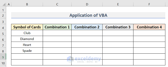
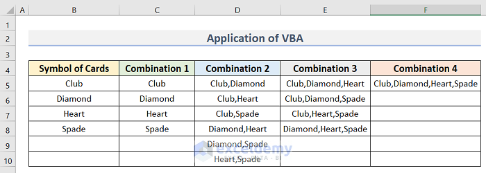
- Arrange a dataset similar to the below image. We have the Symbol of Cards dataset in Column B, and Combination 1, Combination 2, Combination 3, and Combination 4 in Columns C, D, E, and F.
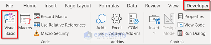
- Go to the Developer tab and select Visual Basic.
The VBA editor will appear.
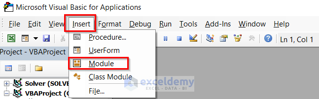
- Select Insert >> Module to open a VBA Module.
- Enter the following code in the VBA Module:
Sub DeterminePermutations()
Dim InValue1 As Variant
Dim OutValue1 As Range
Dim xDict As Object
Dim xlF As Long
Dim xCha As String
InValue1 = Range("B5:B8").Value
Set OutValue1 = Range("C4")
xCha = ","
For xlF = 1 To UBound(InValue1)
    Set xDict = CreateObject("Scripting.Dictionary")
    xDict(0) = "Combination " & xlF
    Call JoinValue(InValue1, xDict, 0, xlF, 0, "", xCha)
    OutValue1.Offset(0, xlF - 1).Resize(xDict.Count).Value = WorksheetFunction.Transpose(xDict.Items)
    Set xDict = Nothing
Next
End Sub
Sub JoinValue(ByRef prValue, ByRef poDictionary, ByRef pvLevel, ByVal pxMaxLevel, ByVal pdIndex, ByVal pxValue, ByVal pxChar)
Dim xlF As Long
If pvLevel = pxMaxLevel Then
    poDictionary(poDictionary.Count + 1) = pxValue
    Exit Sub
End If
For xlF = pdIndex + 1 To UBound(prValue)
    If pxValue = "" Then
        Call JoinValue(prValue, poDictionary, pvLevel + 1, pxMaxLevel, xlF, prValue(xlF, 1), pxChar)
    Else
        Call JoinValue(prValue, poDictionary, pvLevel + 1, pxMaxLevel, xlF, pxValue & pxChar & prValue(xlF, 1), pxChar)
    End If
Next
End Sub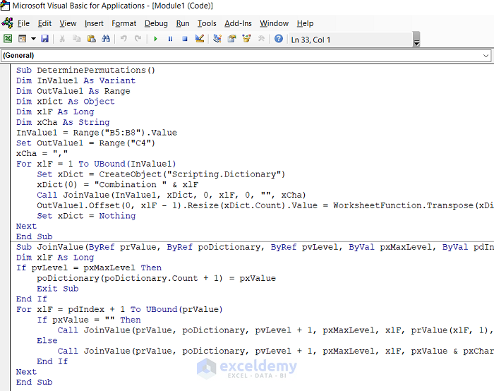
- Press the Run or F5 button to run the code.
The results are as follows:
Read More: How to Perform Permutation and Combination in Excel VBA
Download Practice Workbook
<< Go Back to Excel PERMUT Function | Excel Functions | Learn Excel
Get FREE Advanced Excel Exercises with Solutions!
