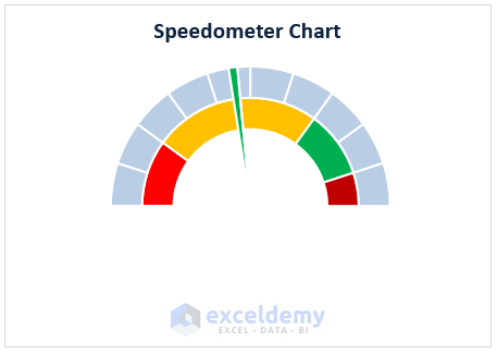
A Speedometer Chart is a gauge where a needle points to specific values at a given point in time. Users create Speedometer Charts in Excel to track value changes. Although there is no direct feature to create a Speedometer Chart in Excel, we can achieve it by inserting a Combo Chart.
Dataset Overview
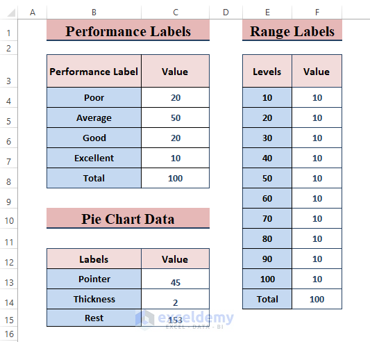
We’ll use the below 3 datasets for the 3 types of properties of a Speedometer Chart.
Speedometer Chart and Its Components
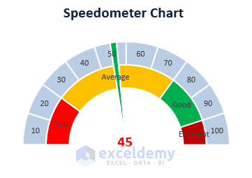
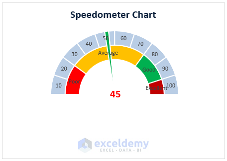
A gauge chart with a needle indicating the ongoing change in values is known as the Speedometer Chart.
Performance Labels: Multiple types of performance labels, such as Poor, Average, Good, etc., are indicated on the dial.
Range Labels: For displaying the instant speed, a Speedometer Chart has range labels on it for displaying the instant speed.
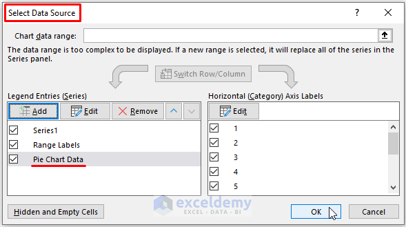
Pie Chart Data: To indicate a certain point or number, a different data source needs to be assigned to create the indicator needle on the chart.
A Speedometer Chart is a Combo Chart. Users need to insert two Doughnuts and a Pie Chart to create a Speedometer Chart. Follow the below steps to insert a speedometer chart into Excel.
Step 1 – Setting up Data to Create a Speedometer Chart
- Each Speedometer Chart has three components, and users need an individual dataset for each of them. Enter the values for each component as shown in the image.

Step 2 – Inserting Doughnut Charts in Excel
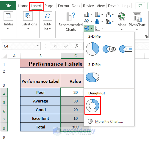
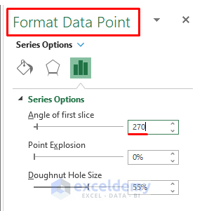
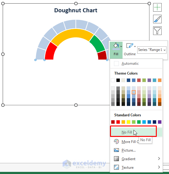
- You can choose any desired color for each portion within the doughnut chart as the Fill Color by right-clicking on the chart. Additionally, use the Format Data Point option from the Context Menu.
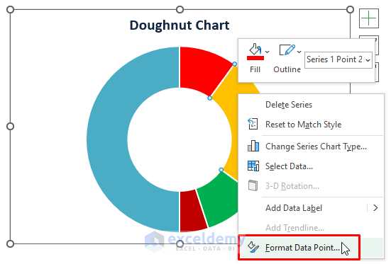
- In the Format Data Point side window, set the Angle of the first slice to 270°.
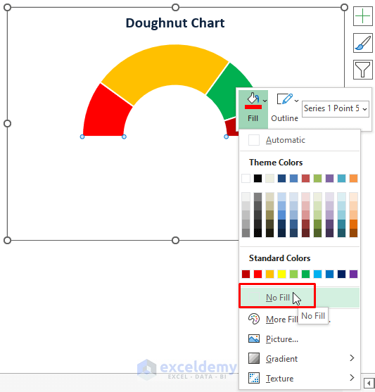
- Select the other half (same colored) and choose No Fill as the Fill Color for that portion.
Read More: How to Create a Gauge Chart in Excel
Step 3 – Inserting a Range Labels Doughnut Chart
- Performance Labels represent different types of ranges (e.g., Poor, Good, Average, or Others). To indicate an exact value, users need to add Range Labels to the chart.
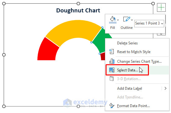
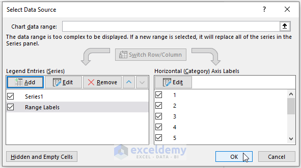
- Right-click on the chart and choose Select Data.
- In the Select Data Source dialog box, click Add (under Legend Entries (Series)).
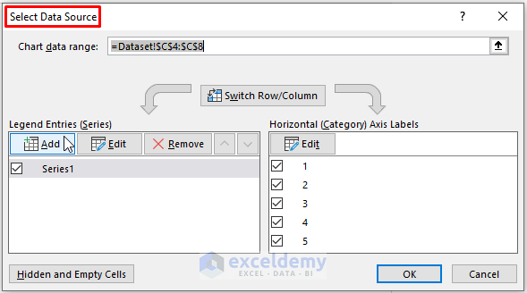
- Assign the respective ranges in the Edit Series dialog box, then click OK.
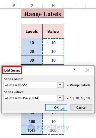
- Back in the Select Data Source dialog box, you’ll see the newly added Range Labels.
- Click OK.
- Since we trimmed the first slice at 270°, select that portion and fill it with No Fill.
Step 4 – Inserting a Pie Chart (Combo Chart)
- Adding data sources to the doughnut chart results in two doughnut charts with individual data sources.
- Follow Step 3 to add another data source and insert a Pie Chart.
- Click OK.
- Right-click on the newly inserted chart and choose Change Series Chart Type… from the Context Menu.
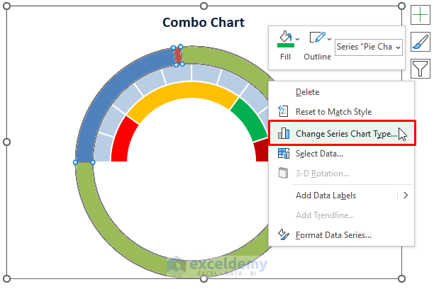
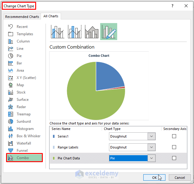
- In the Change Chart Type window, Excel automatically selects the Combo Chart under Recommended Charts.
- Select a Pie Chart for the Pie Chart Data Series and click OK.
- Cut the first slice at 270° for the Pie Chart (the Pointer reverses). Select the entire portion of the Pie Chart, right-click, and choose No Fill as the Fill Color.
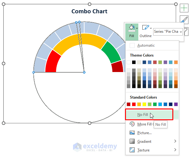
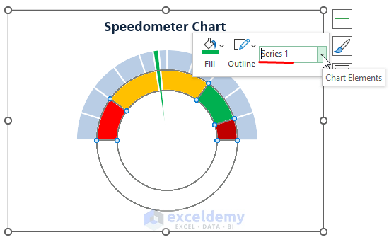
- Select another fill color (e.g., Green) for the needle.
Step 5 – Adding Data Labels to the Speedometer Chart in Excel
- After inserting all three components (Doughnut Charts and Pie Chart), users need to assign data labels to individual portions.
- Right-click on the chart, then select any of the data sources (Series 1, Performance Labels, Range Labels, or Pie Chart Data).
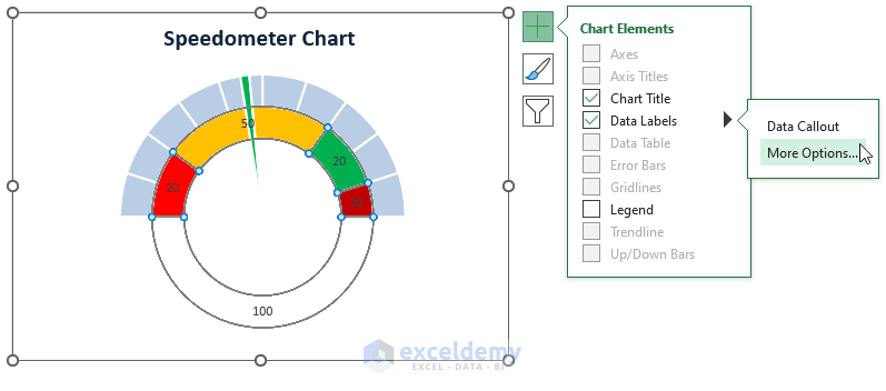
- Click on Chart Elements, then tick Data Labels and choose More Options.
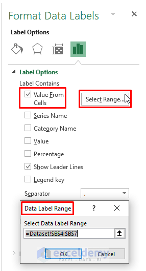
- The Format Data Labels window appears. Under Label Options, tick Value from Cells, and then select the range for the data labels.
- The Data Labels dialog box appears. Insert the Performance Labels (e.g., Poor, Average, Good) as data labels.
You’ll see that all the Performance Labels values are now inserted as data labels.
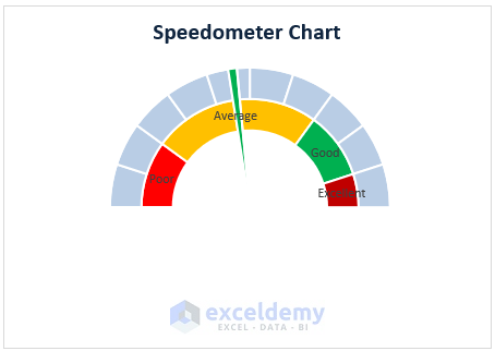
- Repeat the above process for the other two data sources (Range Labels and Pie Chart Data) to complete your Speedometer Chart. Additionally, consider adding a Text Box (Insert > Text > Text Box) with a number to indicate the current speed on the chart.
Download Excel Workbook
You can download the practice workbook from here:
Related Articles
<< Go Back to Excel Charts | Learn Excel
Get FREE Advanced Excel Exercises with Solutions!

This is great, however, what is the formula for where the needle points? You can clearly see even in your graph that the chart says 45 and the needle is pointing to around 55. The further you go toward 100, the bigger the difference. So how do you get it to match?
Hello Kevin,
Here the needle is pointing at 45 but as we kept the number inside the pie chart may seem 55 but actual point is 45. For your better understanding I am attaching another article for the clear view. Sorry for the confusion.
Please read this article from step 6: How to Create a Gauge Chart in Excel (With Easy Steps)
You can watch these two images to clear the confusion.
Regards
ExcelDemy