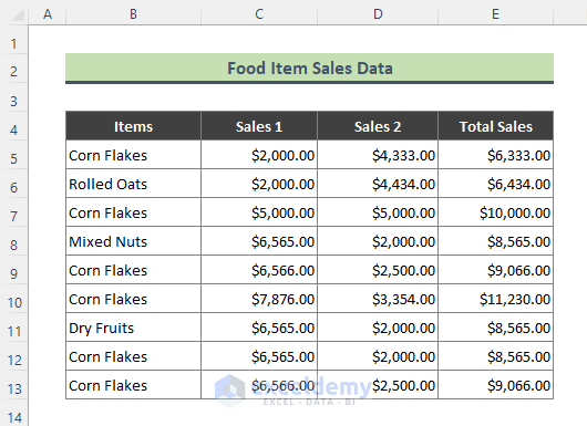
Usually, we can use the COUNTA function to get the count of existing rows in a dataset. However, when rows are hidden manually or through applying the Filter option, the COUNTA function does not give the visible row count. We will show you other Excel functions to get the count of only visible cells. To illustrate, we have a dataset containing some food items’ sales data.
Method 1 – Using Excel SUBTOTAL Function to Count Only Visible Cells
Let’s apply a Filter to the dataset and then calculate the visible rows.
Steps:
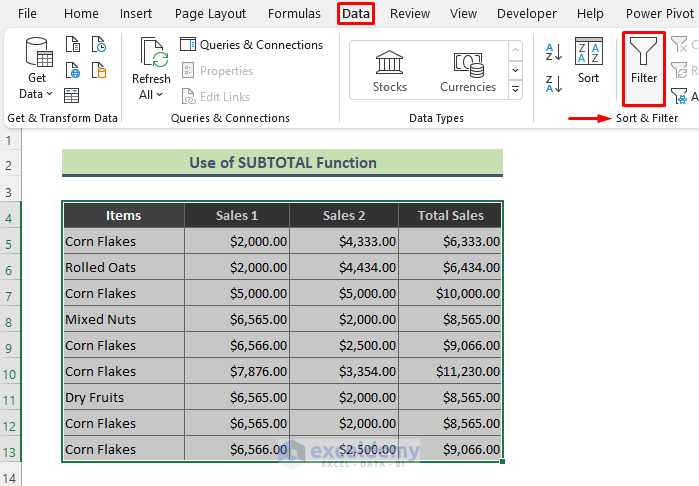
- Select the dataset (B4:E13) and go to Data > Filter or press Ctrl + Shift + L to apply filtering in the dataset.
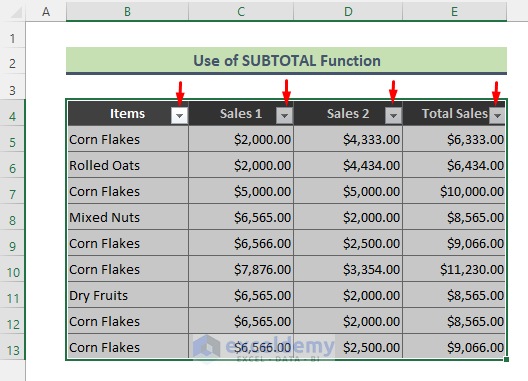
- The filtering drop-down icon is visible below.
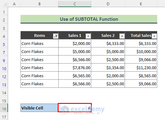
- We have filtered sales data for Corn Flakes (see screenshot).
- Copy this formula in Cell C16 and press Enter:
=SUBTOTAL(3,B5:B13)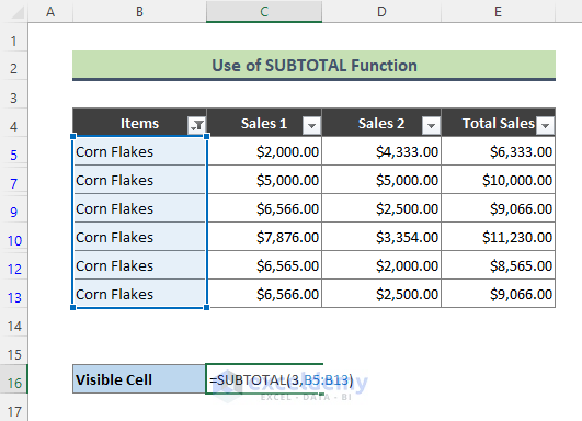
- You will get the row count only for Corn Flakes which is 6.
In the above formula, 3 tells the function what type of count to perform in the range B5:E13.
⏩ Note:
- You can use the below formula to find the count of all cells:
=SUBTOTAL(103,B5:E13)Method 2 – Counting Visible Excel Rows Only with Criteria (Combination of Excel Functions)
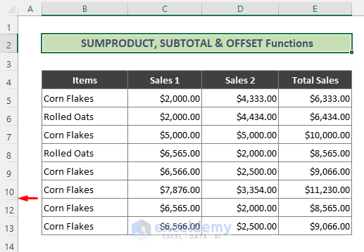
We manually hid row 11 of the dataset and will calculate the count of visible rows containing Rolled Oats using a combination of Excel functions.
Steps:
- Copy the following formula in Cell C18 and hit Enter:
=SUMPRODUCT((B5:B13=C16)*(SUBTOTAL(103,OFFSET(B5,ROW(B5:B13)-MIN(ROW(B5:B13)),0))))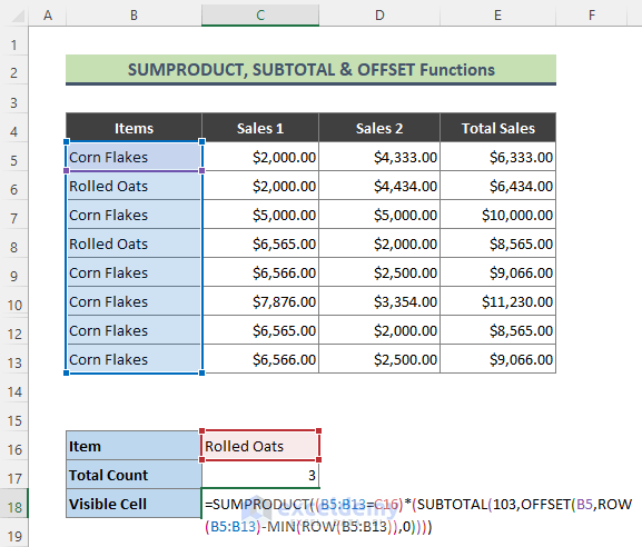
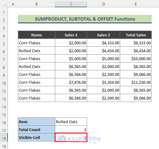
- Here is the cell count of visible cells for Rolled Oats.
How Does the Formula Work?
- (B5:B13=C16)
The above part of the formula returns: {FALSE;TRUE;FALSE;TRUE;FALSE;FALSE;TRUE;FALSE;FALSE}
- ROW(B5:B13)
Here, the ROW function returns the number of rows in the range B5:E13.
{5;6;8;9;10;11;12;13}
- MIN(ROW(B5:B13))
Then the MIN function gives the smallest row in the range B5:E13.
- (SUBTOTAL(103,OFFSET(B5,ROW(B5:B13)-MIN(ROW(B5:B13)),0)))
After that, the above part of the formula returns:
{1;1;1;1;1;1;0;1;1}
- SUMPRODUCT((B5:B13=C16)*(SUBTOTAL(103,OFFSET(B5,ROW(B5:B13)-MIN(ROW(B5:B13)),0))))
The formula returns {2}, which is the number of visible cells containing Rolled Oats.
Method 3 – Applying Excel AGGREGATE Function to Count Only Visible Cells
Let’s count the visible rows from the filtered dataset for Corn Flakes.
Steps:
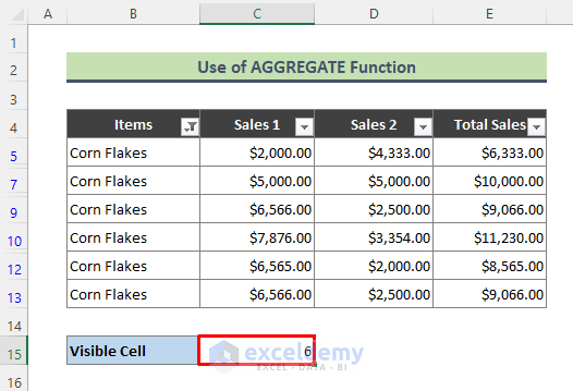
- Copy the below formula in Cell C15 and press Enter:
=AGGREGATE(3,3,B5:B13)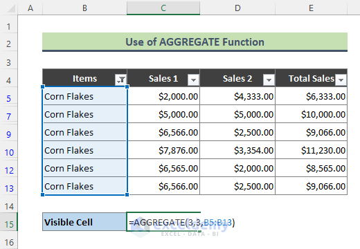
- You will get the count of visible rows only.
Method 4 – Combining COUNTA, UNIQUE, and FILTER Functions to Calculate Unique Visible Cells
Let’s count the visible rows that contain unique values. We are going to use the above dataset where row 11 is hidden.
Steps:
- Add an extra column ‘Visible’ to the dataset. We have used the below formula for the helper column:
=SUBTOTAL(3,B5)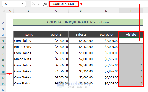
- The extra column added above shows the visibility of the respective rows.
- Calculate the total count of the visible rows by using the below formula:
=SUM(F5:F13)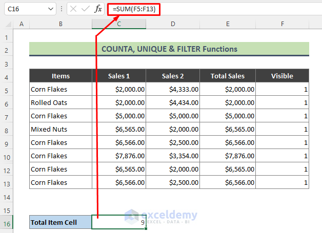
- Type the below formula in Cell C17 and hit Enter:
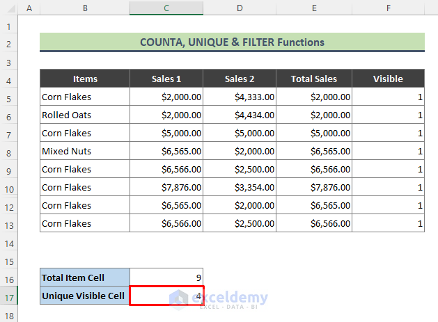
=COUNTA(UNIQUE(FILTER(B5:B13,F5:F13)))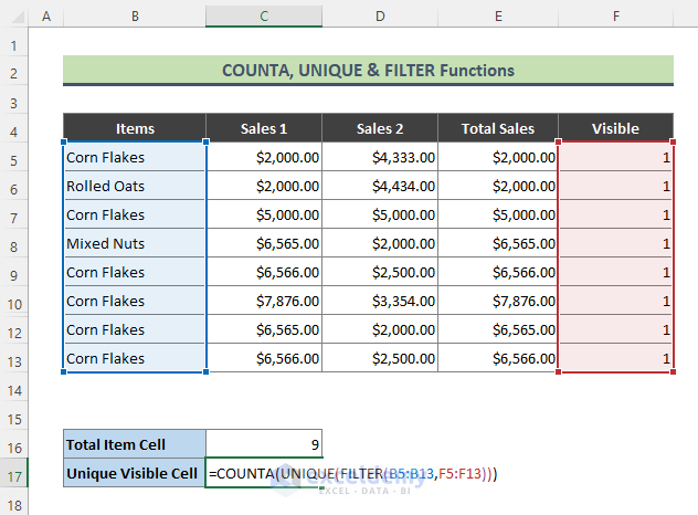
- The above formula will return the below result.
How Does the Formula Work?
- FILTER(B5:B13,F5:F13)
In this part, the FILTER function filters all the food items that are visible and returns:
{“Corn Flakes”;”Rolled Oats”;”Corn Flakes”;”Mixed Nuts”;”Corn Flakes”;”Corn Flakes”;”Dry Fruits”;”Corn Flakes”;”Corn Flakes”}
- UNIQUE(FILTER(B5:B13,F5:F13))
Then the UNIQUE function returns the unique food items from the filtered items which are:
{“Corn Flakes”;”Rolled Oats”;”Mixed Nuts”;”Dry Fruits”}
- COUNTA(UNIQUE(FILTER(B5:B13,F5:F13)))
In the end, the COUNTA function returns the count of visible unique food items as below.
{4}
⏩ Note:
- Remember you can use this formula only in Excel 2021 and Microsoft 365 as UNIQUE and FILTER functions are not available in older versions of Excel.
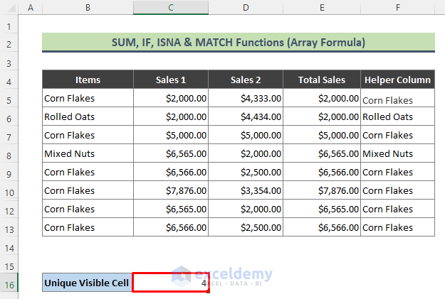
Method 5 – Joining Excel SUM, IF, ISNA, and MATCH Functions to Count Unique Visible Cells
Similarly to the previous method, we will calculate the visible unique values in Excel using an array formula.
Steps:
- Use the below formula in the helper column. This formula is entered as an array (the result is outlined in blue color as below).
=IF(SUBTOTAL(3,OFFSET(B5:B13,ROW(B5:B13)-MIN(ROW(B5:B13)),,1)),B5:B13,"")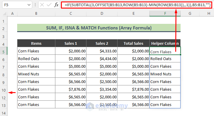
- Type the following formula in Cell C16 and press Enter:
=SUM(N(IF(ISNA(MATCH("",F5#,0)),MATCH(B5:B13,B5:B13,0),IF(MATCH(F5#,F5#,0)=MATCH("",F5#,0),0,MATCH(F5#,F5#,0)))=ROW(B5:B13)-MIN(ROW(B5:B13))+1))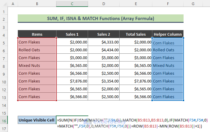
- You will find that there are four unique food items present in the visible rows of our dataset.
How Does the Formula Work?
This formula is quite lengthy, I have explained it in brief.
- IF(ISNA(MATCH(“”,F5#,0)),MATCH(B5:B13,B5:B13,0),IF(MATCH(F5#,F5#,0)=MATCH(“”,F5#,0),0,MATCH(F5#,F5#,0)))
Initially, the above portion of the formula returns:
{1;2;1;4;1;1;7;1;1}
- ROW(B5:B13)-MIN(ROW(B5:B13))+1)
Next, this part of the formula returns:
{1;2;3;4;5;6;7;8;9}
- SUM(N(IF(ISNA(MATCH(“”,F5#,0)),MATCH(B5:B13,B5:B13,0),IF(MATCH(F5#,F5#,0)=MATCH(“”,F5#,0),0,MATCH(F5#,F5#,0)))=ROW(B5:B13)-MIN(ROW(B5:B13))+1))
In conclusion, the above formula returns:
{4}
Download Practice Workbook
You can download the practice workbook that we have used to prepare this article.
<< Go Back to Count Cells | Formula List | Learn Excel
Get FREE Advanced Excel Exercises with Solutions!
