Method 1 – Use the Format Cells Command to Convert Fraction to Decimal in Excel
1.1 Converting into General Format
Steps:
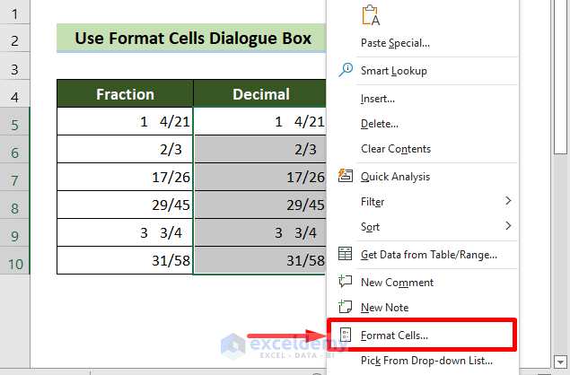
- Copy the fraction numbers and paste them into the cells where you want to convert them to decimals. Select all the cells and press the right-click button. From the context menu, click on the Format Cell option.
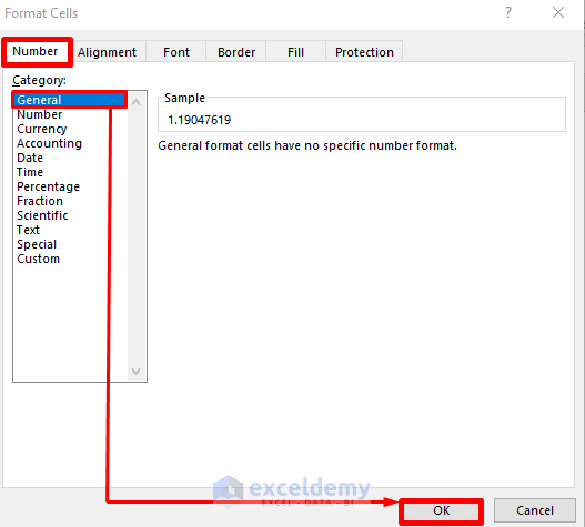
- The Format Cells window will appear. Go to the Number tab. Select the General option from the Category list. Click the OK button.
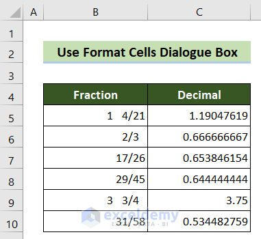
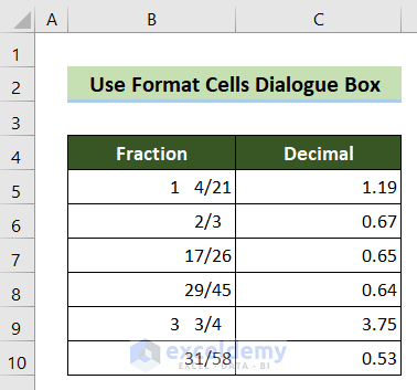
All the fractions will be converted to decimals. You can not choose any formatting for the decimal results. The result sheet will look like this.
1.2 Converting into Number Format
Steps:
- Copy the fraction numbers and paste them into the cells where you want to convert to decimal at first. Select all the cells and press the right-click button. Click the Format Cell option from the context menu.

- The Format Cells window will appear. Go to the Number tab. Select the Number option from the Category list. Click the OK button.
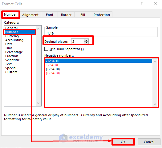
- Choose the formatting for the decimal numbers here. Choose decimal places, negative numbers format, use of thousands separator, etc in this category.
All the fractions will be converted to decimals. Choose your desired formatting for the decimal results. The result sheet will look like this.
Method 2 – Use the Number Format Icon
Steps:
- Copy the fraction numbers and paste them into the cells where you want to convert to decimal at first. Select all the cells and go to the Home tab. Go to the Number group. Click on the Number Format icon situated at the bottom-right corner of the group.
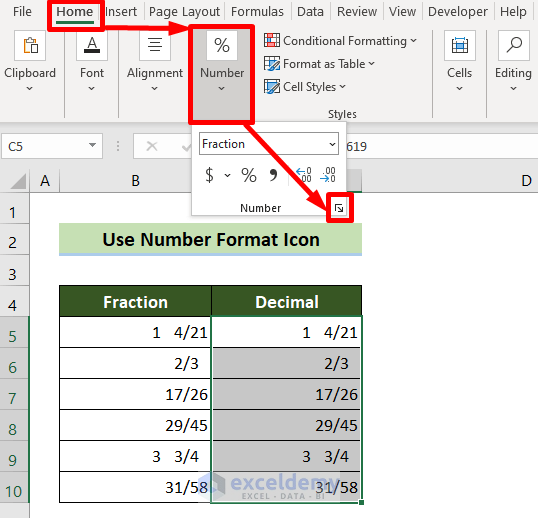
- The Format Cells window will appear. As per your requirements, follow step 2 from the 1.1 method or steps 2 and 3 from the 1.2 method.
You will get your fractions converted into decimals.
Convert Fraction in Text Format to Decimal in Excel
Case 1: If the Fractions Are Proper
Steps:
- Select the cell where you want to get your converted decimal result. We want to convert the B6 cell fraction data converted to decimal.
- Put the following formula in the result cell.
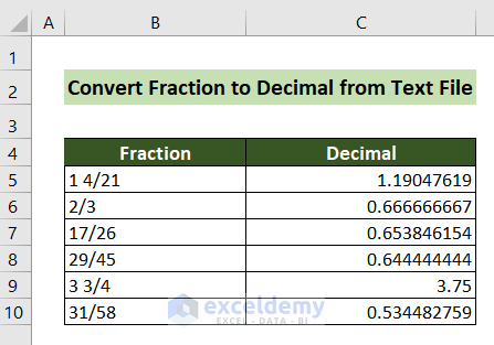
=LEFT(B6,SEARCH("/",B6)-1)/MID(B6,SEARCH("/",B6)+1,99)Press the Enter button. Drag the fill handle downward to copy the formula.
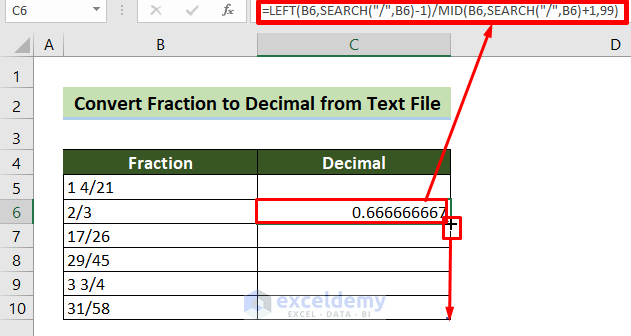
You can convert fractions to decimals from a text file.
Case 2: If the Fractions Are Mixed
Steps:
- Select the cell where you want to get your converted decimal result. We want to convert the B5 cell mixed fraction data converted to decimal.
- Put the following formula in the result cell.
=IF(ISERROR(SEARCH(" ",B5)),LEFT(B5,SEARCH("/",B5)-1)/MID(B5,SEARCH("/",B5)+1,99),LEFT(B5,SEARCH(" ",B5)-1)+MID(B5,SEARCH(" ",B5)+1,SEARCH("/",B5)-1-SEARCH(" ",B5))/MID(B5,SEARCH("/",B5)+1,99))
Press the Enter button. Drag the fill handle downward to copy the formula.
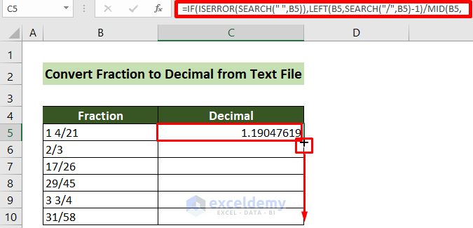
Convert fractions to decimals from a text file. The result will look like this.
Download Practice Workbook
You can download and practice from our workbook here.
Related Articles
- [Solved!] Fraction Changing to Date in Excel
- How to Add a Stacked Fraction in Excel
- How to Format Fraction to Percentage in Excel
<< Go Back to Fraction in Excel | Number Format | Learn Excel
Get FREE Advanced Excel Exercises with Solutions!

Sometimes mixed fractions are written with the ASCII 160 (non-breaking space) character instead of the usual ASCII 32 character that Excel recognizes as ” “. If you get a *VALUE! error, you need to use “CHAR(160)” instead of ” ” in the formula, or clean up your text with a find and replace operation before applying the formula.
Hi, ERIC!
Thank you for your valuable feedback.
You have pointed out a nice thing. When the #VALUE! error happens in this regard, it is better to use the find and replace feature to replace ” ” with CHAR(160) before applying the formula.
Regards,
Tanjim Reza
Good day, this is indeed awesome tips. Can you help me getting the correct formula for time worked when people clock in and out but only get paid for set hours? e.g, clock in 06:20 – clock out 16:25,but only get paid from 07:00 to 16:00,less 15min for lunch? (they get 45min lunch, but they wanted 1 hour lunch so they sacrifice 15min).thus they get paid only for 8.75hours. My challenge is that it must be displayed as 8.75 and not 8,45.
Second challenge :
My hours must work as quarters example
15min must show as 0.25
30min must show as 0.5
45min must show as 0.75
I followed various tries but it does not work the way I need it to work.
If a person’s total time spend is 8hours and 17 min I need a formula yo show it as 8.25 (17min as a fraction of. 25)
If he is Kate and clocks in at 09:22 and clock out at 16:00 his hours to be paid wil be ((16:00-09:22)less 15min) displayed as 6.23, but I need to get it to the closest fraction display as 6.25.(the nearest quarter on the clock)
If it was a weekend this hours will be 6.38 but must be displayed as 6.75 (the nearest quarter on the clock).
Is the above possible with formula for weekdays and different formula for weekends where there is no deduction of 15min for lunch time? Thanking you in advance for your help and time.
Hi RINA,
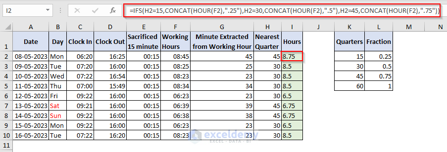
Thanks for your comment. Per your comment, we have tried implementing the conditions in our dataset. You can see the result below:
Here, we have used the formula below in Cell I2:
=IFS(H2=15,CONCAT(HOUR(F2),".25"),H2=30,CONCAT(HOUR(F2),".5"),H2=45,CONCAT(HOUR(F2),".75"))According to one of your conditions (in case of Kate), you wanted 6:23 to be displayed as 6.25. But if you want to display time to the nearest quarter on the clock, it gives 6.5. You can check out the Excel file from the link below:
Answer.xlsx
It will be easier for us to give a proper solution if you send us an Excel file with the desired outputs. You can send the Excel file to my email: [email protected]. Please let us know if you have any other queries.
Regards
Mursalin,
Exceldemy.