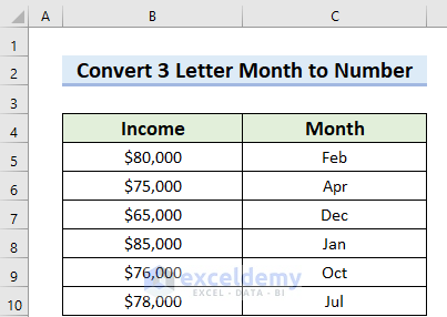
We’ll use the following simple dataset with income over a few months.
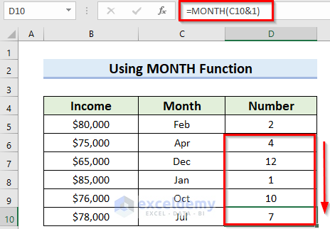
Method 1 – Using the MONTH Function to Convert a 3-Letter Month to Number in Excel
Steps:
- Select the first result cell. We used D5.
- Insert the following formula.
=MONTH(C5&1)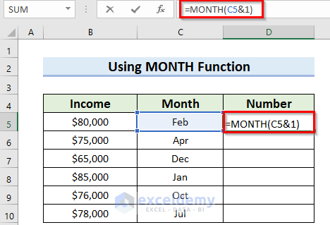
Formula Breakdown
- Here, the MONTH function will return a month as a number of 1 (January) to 12 (December).
- C5&1: Here, Ampersand(&) combines Month nad value which denotes a date.
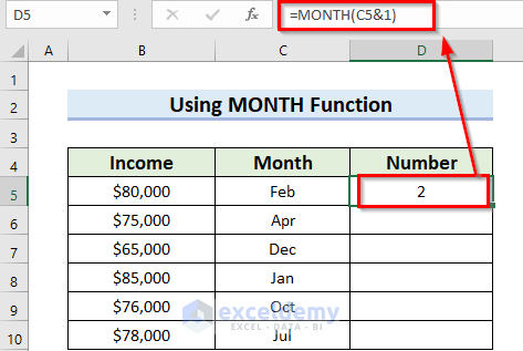
- MONTH(C5&1): will return the month value of February as 2.
- Hit Enter.
- Drag the Fill Handle icon to paste the used formula to the other cells of the column or use Excel keyboard shortcuts Ctrl + C and Ctrl + V to copy and paste.
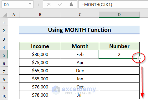
You will get all the converted Month values.
Read More: How to Convert Month to Number in Excel
Method 2 – Applying MONTH and DATEVALUE Functions
Steps:
- Select the first result cell. We used D5.
- Insert the following formula.
=MONTH(DATEVALUE(C5&1))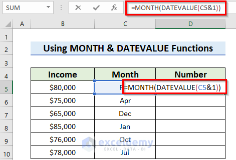
Formula Breakdown
- C5&1 = Feb1: Here, Ampersand(&) combines the value of C5 and 1.
- DATEVALUE(C5&1)=44592: The DATEVALUE function converts the text to a numerical value which represents a date
- MONTH(DATEVALUE(C5&1)) = 2: Finally, the MONTH function give the month value of the date.
- Hit Enter.

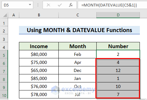
- Drag the Fill Handle icon to AutoFill the corresponding data in the rest of the cells D6:D10.
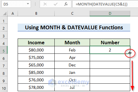
You will see all the converted months in a numerical format.
Method 3 – Using MONTH and LEFT Functions
Steps:
- Select the first result cell. We used D5.
- Insert the following formula.
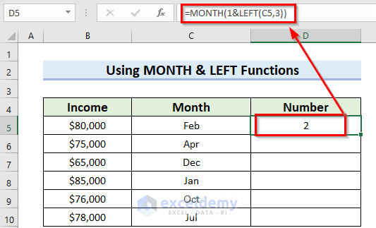
=MONTH(1&LEFT(C5,3))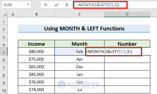
Formula Breakdown
- LEFT(C5,3)= Feb: The LEFT function will extract the leftmost 3 characters of the value of the C5 cell.
- 1&LEFT(C5,3) = 1Feb: Now, Ampersand(&) adds 1 in front with the previous output to make a date.
- MONTH(1&LEFT(C5,3)) = 2: Finally, the MONTH function will extract the month value from the date.
- Hit Enter.
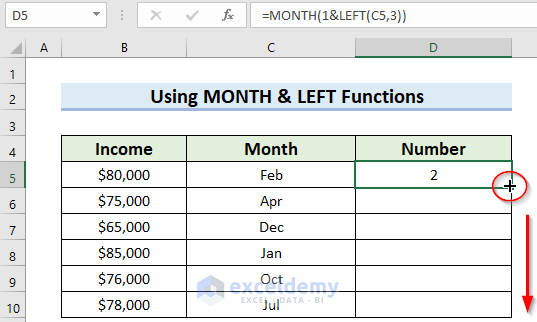
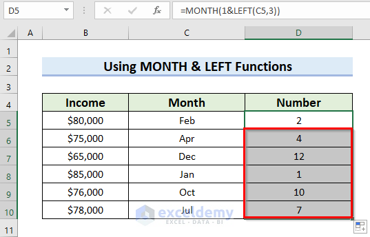
- Drag the Fill Handle icon to AutoFill the corresponding data in the rest of the cells D6:D10.
Here’s the result.
Method 4 – Using the MONTH Function with Symbol
You can not only use the functions but also use the Double Hyphen (–) symbol to convert the 3 letter Month to a number in Excel. In addition, you can combine the MONTH functions with the Double Hyphen (–) symbol. The steps are given below.
Steps:
- Select the first result cell. We used D5.
- Insert the following formula.
=MONTH(--(C5&1))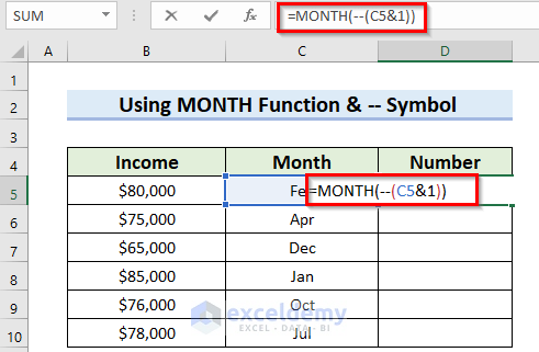
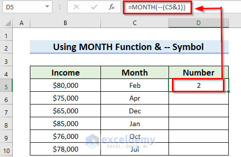
Formula Breakdown
- C5&1 = Feb1: Ampersand(&) combines the value of C5 and 1.
- –(C5&1) = 44593: The double hyphen works like the DATEVALUE function to convert the text to a numerical value that represents a date.
- MONTH(–(C5&1)) = 2: Finally, the MONTH function gives the month value of the date.
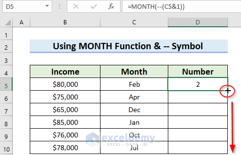
- Hit Enter.
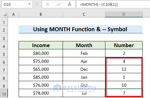
- Now drag the Fill Handle icon to paste the used formula to the other cells of the column or use Excel keyboard shortcuts Ctrl+C and Ctrl+V to copy and paste.
You will get all the converted months.
Read More: Excel Formula to Find Date or Days for Next Month
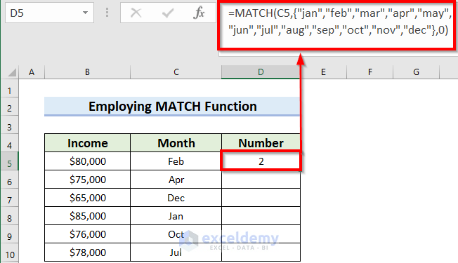
Method 5 – Using the MATCH Function to Convert a 3-Letter Month to Number
Steps:
- Select the first result cell. We used D5.
- Insert the following formula.
=MATCH(C5,{"jan","feb","mar","apr","may","jun","jul","aug","sep","oct","nov","dec"},0)- Hit Enter.
Formula Breakdown
MATCH(lookup_value,lookup_array,[match_type])
- lookup_value = C5: This is the look-up value for which the Match function will search in the array.
- lookup_array = {“jan”,”feb”,”mar”,”apr”,”may”,”jun”,”jul”,”aug”,”sep”,”oct”,”nov”,”dec”} : This is the look-up array where the MATCH
- [match_type] = 0 : The function will search for the exact match.
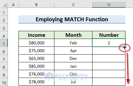
- Drag the Fill Handle icon to paste the used formula respectively to the other cells of the column or use Excel keyboard shortcuts Ctrl + C and Ctrl + V to copy and paste.
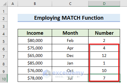
You will get the converted months in the numerical format.
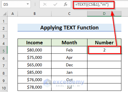
Method 6 – Applying the TEXT Function to Convert a 3-Letter Month to a Number in Excel
Steps:
- Select the first result cell. We used D5.
- Insert the following formula.
=TEXT((C5&1),"m")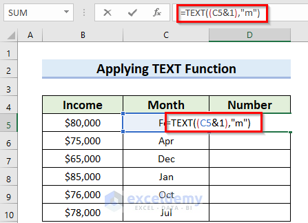
Formula Breakdown
- C5&1 = Feb1 : Ampersand(&) combines the value of C5 and 1.
- TEXT((C5&1),”m”) = 2: The TEXT function will extract the month value from “Feb1”. Here “m” denotes the month value.
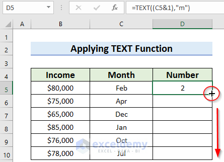
- Hit Enter.
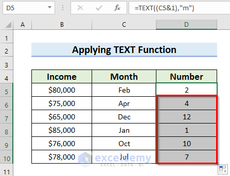
- Dag the Fill Handle icon to AutoFill the corresponding data in the rest of the cells D6:D10.
You will see the converted Months.
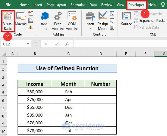
Method 7 – Using a User-Defined Function to Convert a 3-Letter Month to a Number
Steps:
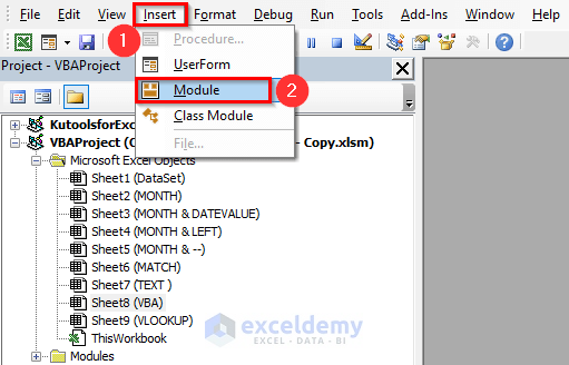
- Choose the Developer tab, then select Visual Basic.
- From the Insert tab, select Module.
- Insert the following Code in the Module.
Function ConvertMonth(givenMonth As String)
    ConvertMonth = Month(DateValue("1 " & givenMonth & " 2022"))
    ConvertMonth = Format(ConvertMonth, "0")
End Function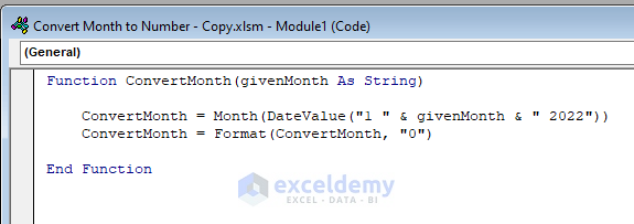
Code Breakdown
- We have created a Function named ConvertMonth.
- We have declared a variable givenMonth as a String to call the Months.
- Using the Month and DateValue functions, we developed the function named ConvertMonth. We have used the Format function to format the result.
- Save the code.
- Go to the Excel worksheet.
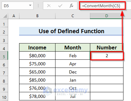
- Select the first result cell. We used D5.
- Insert the following formula.
=ConvertMonth(C5)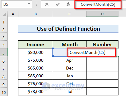
- Hit Enter.
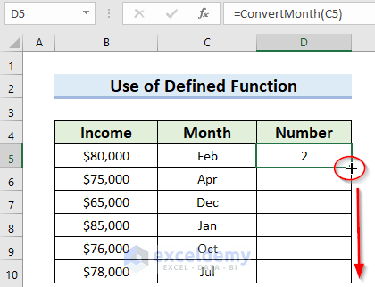
- Drag the Fill Handle icon to AutoFill the corresponding data in the rest of the cells D6:D10.
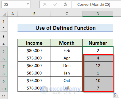
Here’s the result.
Method 8 – Use the VLOOKUP Function to Convert a 3-Letter Month to a Number in Excel
Steps:
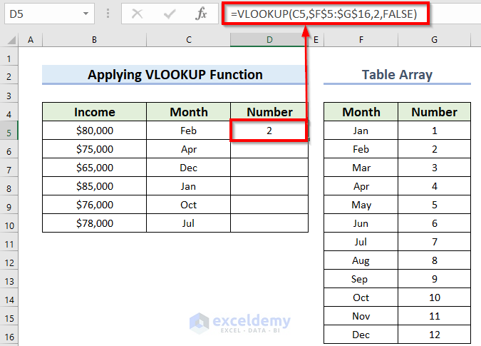
- We created a list of months and the corresponding numbers in columns F and G.
- Select the first result cell. We used D5.
- Insert the following formula.
=VLOOKUP(C5,$F$5:$G$16,2,FALSE)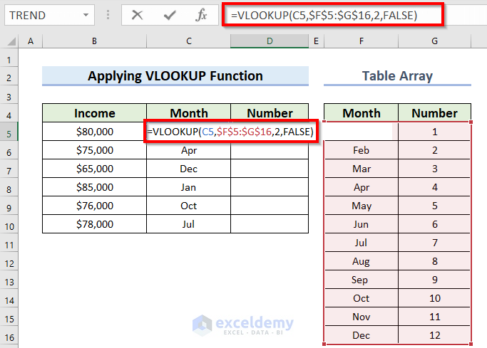
Formula Breakdown
VLOOKUP(lookup_value,table_array,col_index_num,[range_lookup])
- lookup_value = C5: The value that it looks for in the leftmost column of the given table.
- table_array = $F$5:$G$16: The table in which it looks for the lookup_value in the leftmost column.
- col_index_num = 2: The column number in the table from which a value is to be returned.
- [range_lookup] = FALSE: 0 or False for an exact match, 1 or True for a partial match. So, it denotes the exact match for the lookup_value
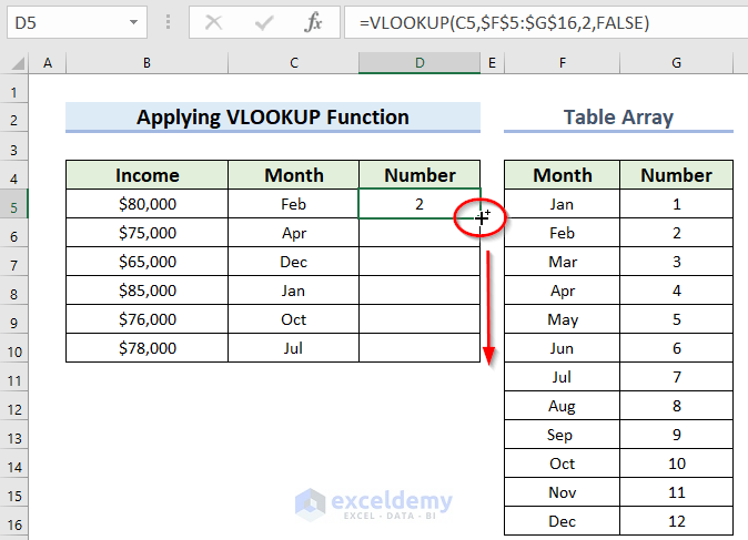
- Hit Enter.
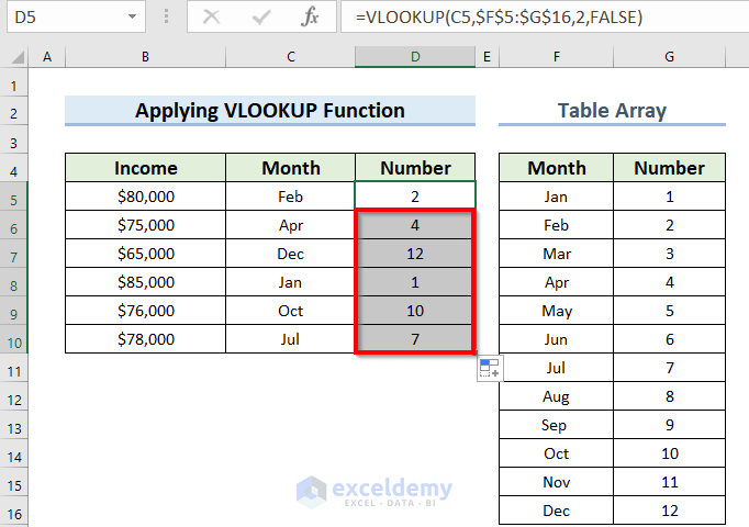
- Drag the Fill Handle icon to AutoFill the corresponding data in the rest of the cells D6:D10.
You will get the converted Months.
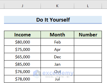
Practice Section
You can practice the explained methods by yourself with the sample dataset.
Download the Practice Workbook
Related Articles
- How to Get First Day of Month from Month Name in Excel
- How to Calculate First Day of Previous Month in Excel
- Excel Formula for Current Month and Year
- How to Get Last Day of Previous Month in Excel
- Excel VBA: First Day of Month
- How to Get the Last Day of Month Using VBA in Excel
<< Go Back to Excel MONTH Function | Excel Functions | Learn Excel
Get FREE Advanced Excel Exercises with Solutions!
