How to Automatically Update One Worksheet from Another Sheet in Excel

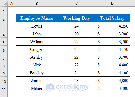
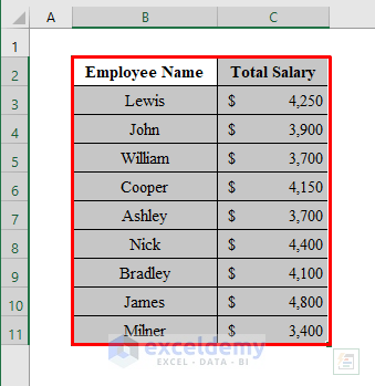
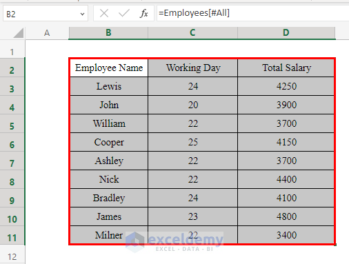
Let’s say we have the following dataset in our source worksheet: Employee Name, Working Day, and Total Salary, and we want to automatically update any changes to this data in another worksheet in Excel. We can do this by using one of the six following methods.

Method 1 – Using the Paste Link Feature

The simplest way to connect and update one worksheet from another is to use the paste link feature in Microsoft Excel. Follow the steps below.

Steps:

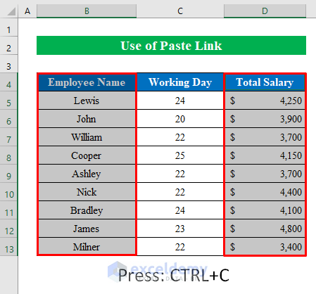
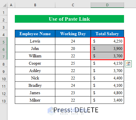
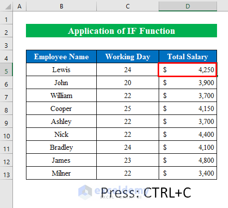
• First, select the list from the table that you want to update in a new worksheet. Here we have chosen cell (B4:B13) and cell (D4:D13).
• Second, press CTRL+C to copy.

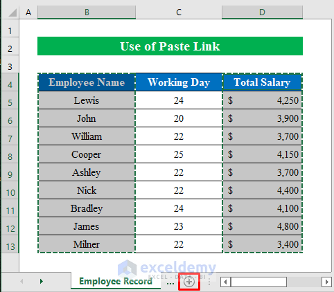
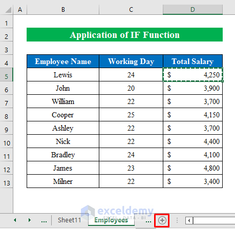
• Next, click the “New Sheet” icon below to create a new worksheet.

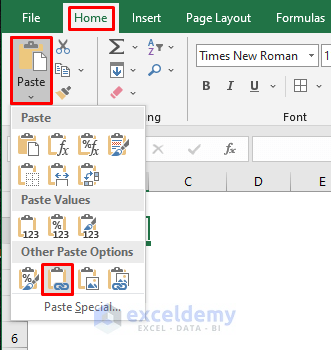
• In the new worksheet, choose a cell (B2) and click on the “Paste Link” under the “Paste” option.

• Your selected data will be copied into the new sheet.

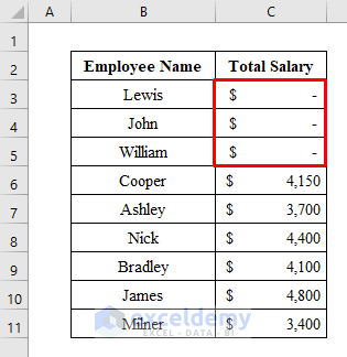
• Let’s check if the data updates automatically or not. Return to the previous worksheet and select cell (D5:D7), then press DELETE on your keyboard.

• Now, if we go back to the new sheet, we will see the data is missing, which confirms an automatic update from the new sheet.

Read More: Transfer Data from One Excel Worksheet to Another Automatically

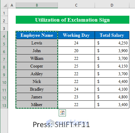
Method 2 – Utilize Exclamation Sign to Update Automatically

Sometimes, you might need to update one worksheet from another manually. To do so, use the exclamation sign (!) on your keyboard.

Steps:

• Select cells (B4:B13) and press CTRL+C to copy.

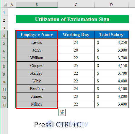
• Click SHIFT+F11 to open a new worksheet in the same workbook.

• Choose a cell (B2) in the new sheet and type the following formula:

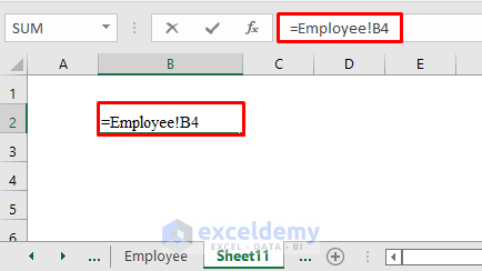
• Press ENTER.
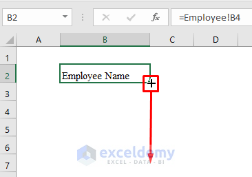
• Here, we will drag down the Fill Handle to fill all the cells.

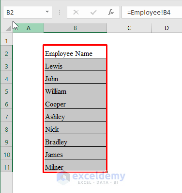
• The column data will update from one worksheet to another sheet.

Read More: How to Link Two Sheets in Excel

Method 3 – Apply IF Function to Automatically Update Data Based on Criteria

The IF function allows you to update worksheets based on criteria being met and is another good method to update one worksheet from another in Excel automatically.

Steps:

• Select a cell (D5) and hit CTRL+C to copy.

• Click the “New Sheet” icon below to create a new worksheet.

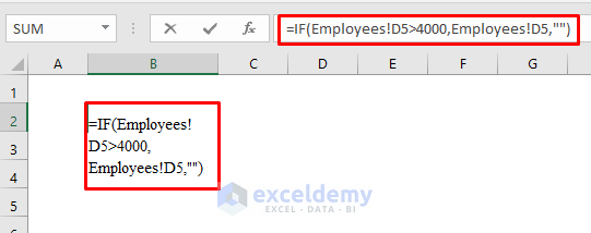
• Inside the newly created sheet, choose a cell (B2) and apply the following formula:

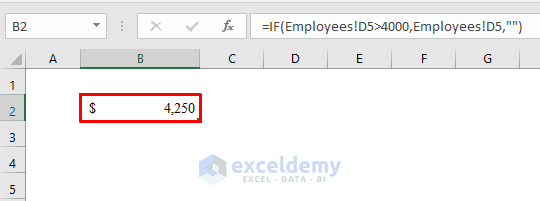
• The IF Function will provide an output if the value in the cell Employees!D5>4000 is more than 4000. Otherwise, the cell will remain blank.

• Hit ENTER.
• You have now successfully updated the value from the previous sheet with the criteria.

Read More: How to Link Sheets in Excel with a Formula

Method 4 – Utilize Drop-Down List to Update the New Sheet Automatically

In the previous methods, we learned how to automatically update cells or columns from one worksheet to another. In this method, we will update the drop-down list from another sheet.

Imagine we have a drop-down list in our worksheet with employee names. Now, we will link this list from our source sheet with another sheet to update it automatically.

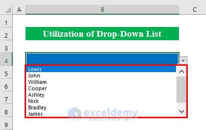
Steps:

• Create a new worksheet, select a cell (B2), and apply this formula:

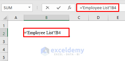
• Press ENTER.
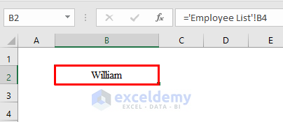
• Go back to the previous sheet and choose any name from the drop-down list. In our example, we selected “William.”

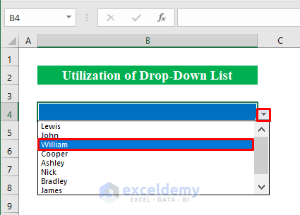
• In the newly created sheet, you will see the name is updated automatically.

Read More: Best Practices for Linking Excel Spreadsheets

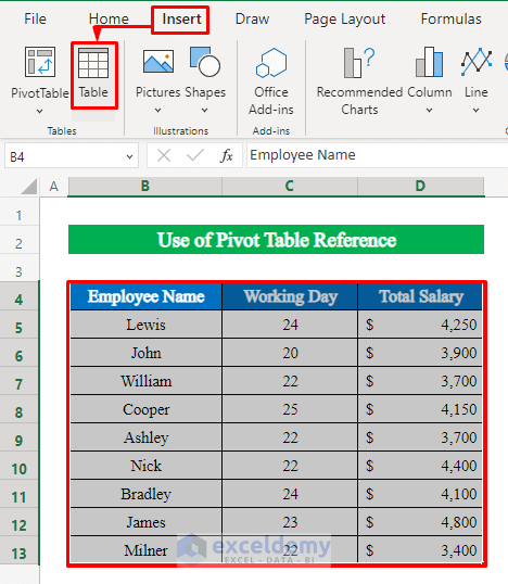
Method 5 – Update Different Sheet Using Pivot Table Reference

Steps:

• Click on “Insert” followed by “Table” and select the list from a worksheet.

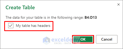
• Check the “My table has header” option and hit OK to continue.

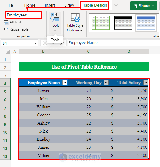
• Select the table, click the “Table Design” option, and name your table.

• Create a new worksheet and type the following formula:

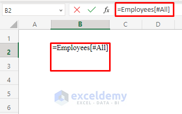
• Hit ENTER, and your complete list will update from one worksheet to another within seconds.

Read More: How to Link a Table in Excel to Another Sheet

Method 6 – Using Power Query Feature

If you want to try another handy method to automatically update one worksheet from another sheet, try using the power query feature.

Step 1:

• Create a table from your dataset.
• Under “Data” select “From Table/Range”.

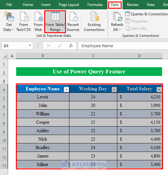
• A new window with the “Power Query Editor” will pop up.
• Hit the “Close & Load” option.

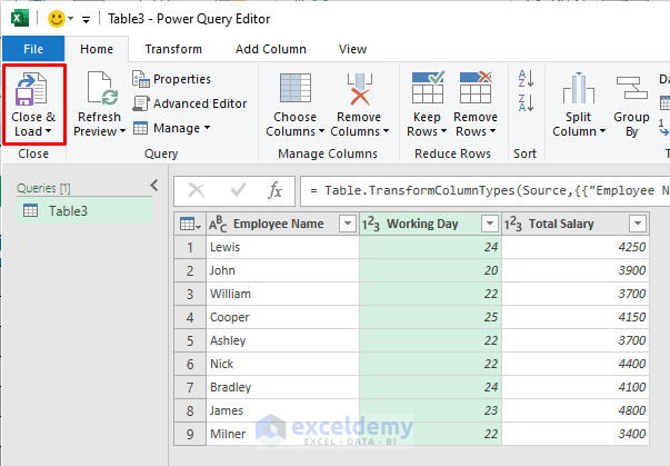
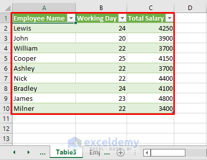
• The selected table will be created in a new worksheet momentarily. Let’s check whether it updates automatically or not.

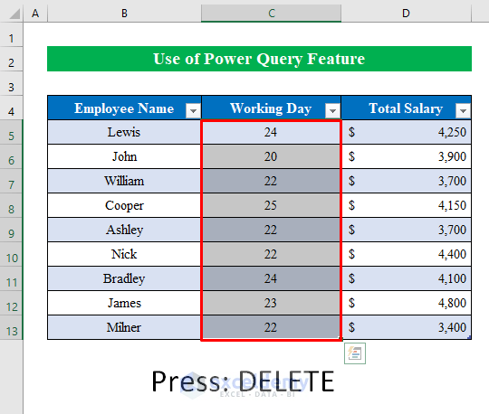
Step 2:

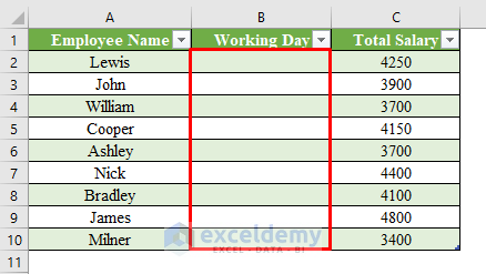
• Select cells (C5:C13) and press DELETE on your keyboard.

• Switch to the newly created worksheet, and under “Data” click “Refresh All”.

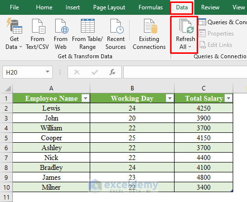
• You have automatically updated one worksheet from another sheet in Excel.

Things to Remember

• In method 5, you won’t be able to use the pivot table reference without Excel 365.

Download Practice Workbook

Download this practice workbook to exercise while you are reading this article.

Related Articles

• How to Reference Cell in Another Excel Sheet Based on Cell Value
• Transfer Specific Data from One Worksheet to Another for Reports
• Linking Excel Sheets to a Summary Page
• How to Make Excel Look Like an Application

<< Go Back To Excel Link Sheets | Linking in Excel | Learn Excel