How to Adjust Row Height to Fit Text in Excel: 6 Suitable Methods

Method 1 – Clicking and Dragging to Adjust Excel Row Height and Fit Text

Steps:

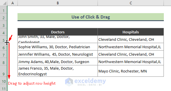
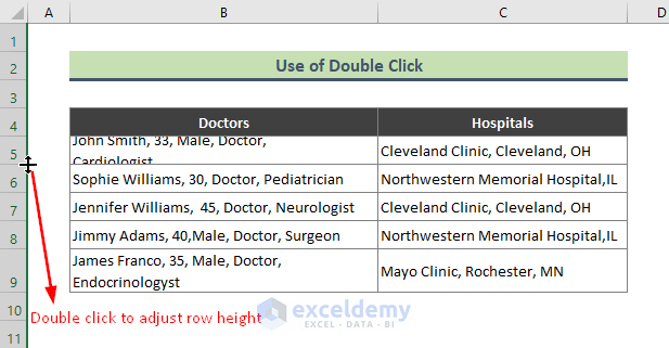
Put the mouse cursor on the border of the row of which you want to change the height.
Drag the bottom border of the row heading.

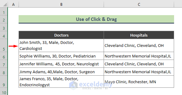
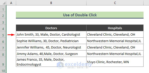
Adjust Excel Row Height Using Click and Drag to Fit Text

The row height is adjusted.

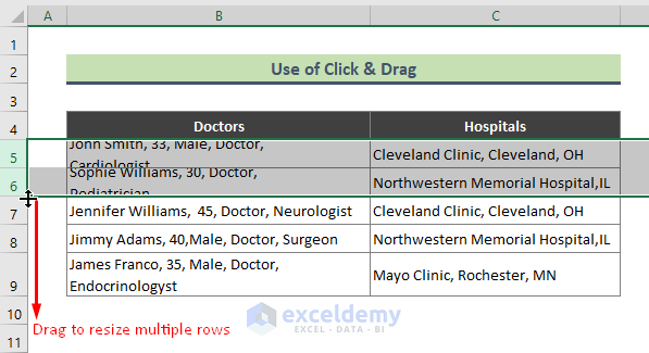
Adjust Excel Row Height Using Click and Drag to Fit Text

Select the rows that have insufficient height.
Drag down the bottom border of any row heading from the selected rows.

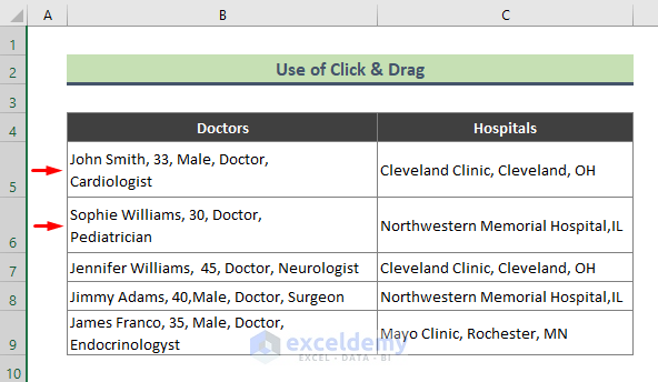
Adjust Excel Row Height Using Click and Drag to Fit Text

You will get the following result.

Method 2 – Using the Mouse to Set Row Height to Adjust Text in Excel

Steps:

Put the cursor on the lower border of the row header of which you want to change the height.
Double-click on it.

Use Mouse to Set Row Height to Adjust Text

Excel will adjust the row height based on the text in it.

Use Mouse to Set Row Height to Adjust Text

If you want to adjust the height of multiple rows, follow the below instructions:

Select the corresponding rows and double-click on the lower border of any of the row headers in the selection.

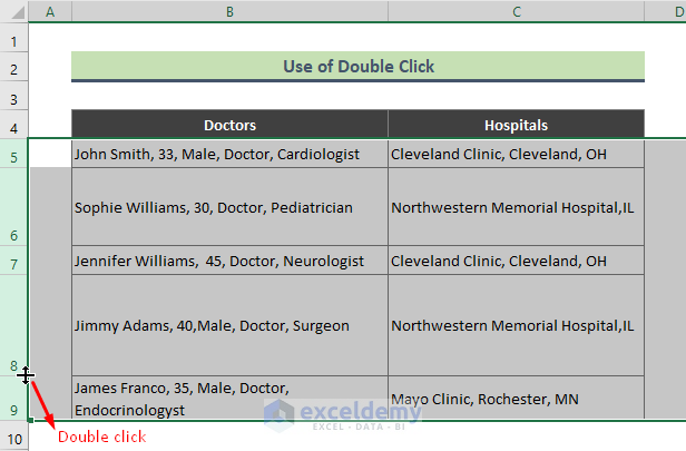
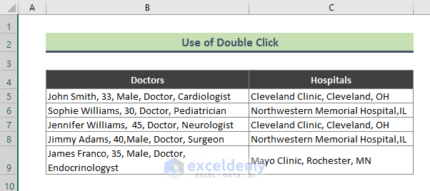
Use Mouse to Set Row Height to Adjust Text

The height of all selected rows is adjusted according to the cell contents.

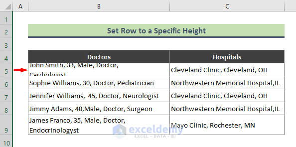
Method 3 – Adjusting the Row to a Specific Height in Excel to Fit Text

Steps:

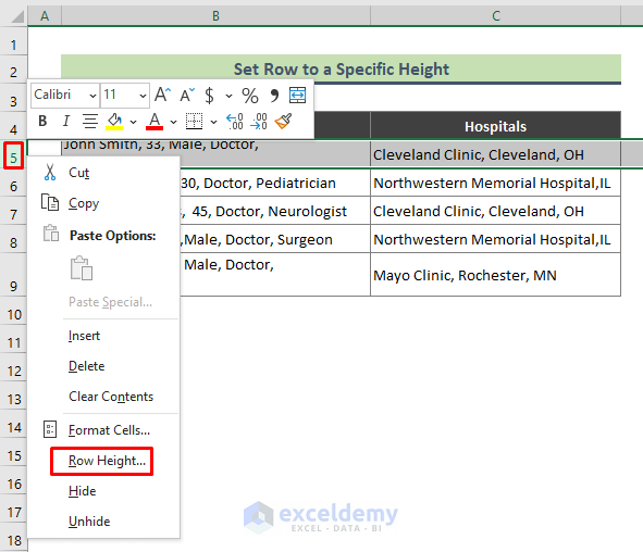
Select the row in which you want to adjust the height.

Adjust Row to a Specific Height to Fit Text in Excel

Right-click on the selected row and select Row Height.

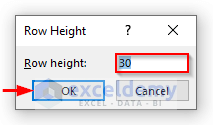
Adjust Row to a Specific Height to Fit Text in Excel

The Row Height dialog appears. In the Row Height field, type the desired height and press OK.

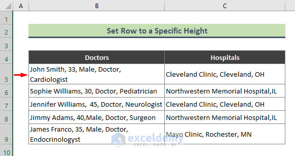
Adjust Row to a Specific Height to Fit Text in Excel

You will get the below result. Row 5 is adjusted to fit the text located in it.

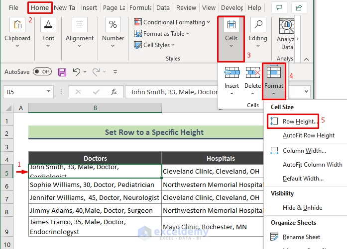
Adjust Row to a Specific Height to Fit Text in Excel

You can use the Home tab to set row height manually. Select the row and go to Home > Cells > Format > Row Height.

Method 4 – Using Home Tab to Autocorrect Row Height to Adjust Text

Steps:

Select the row or the cell that is not adjusted according to the text height.
From Excel Ribbon go to Home > Cells > Format > AutoFit Row Height.

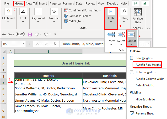
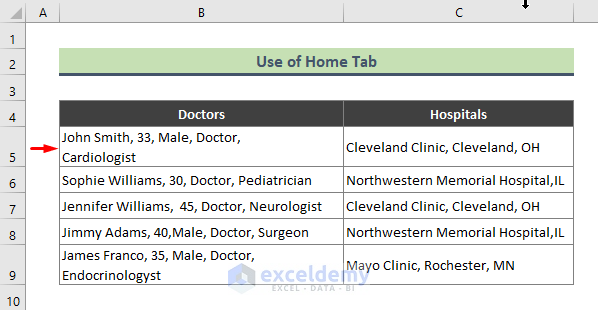
Excel Home Tab to Autocorrect Row Height to Adjust Text

Excel will adjust the row height to fit the text in it.

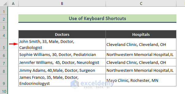
Method 5 – Applying Keyboard Shortcut to Set Row Height to Fit Text

Steps:

Select the row with the insufficient row height.

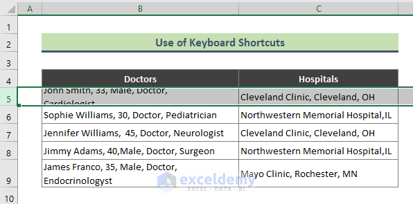
Use Keyboard Shortcut to Set Row Height to Fit Text

Press the following keys one by one to apply the AutoFit Row Height option: Alt + H + O + A

Row 5 is adjusted to its text.

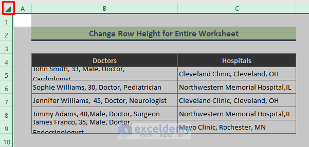
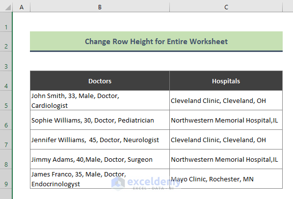
Method 6 – Fitting Text by Changing Row Height for Entire Excel Worksheet

Steps:

Select all the cells in the active worksheet by selecting the small triangle icon at the intersection of the column and row header. Press Ctrl + A + A to select all the cells in a worksheet.

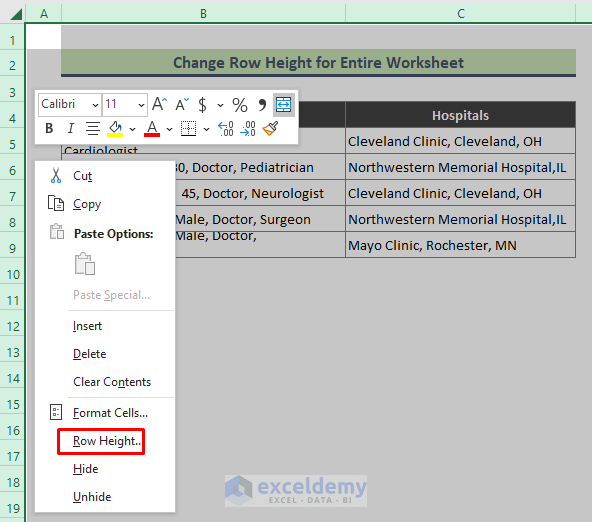
Fit Text by Changing Row Height for Entire Excel Worksheet

Right-click anywhere in the selection and select Row Height.

Fit Text by Changing Row Height for Entire Excel Worksheet

When the Row Height dialog box appears, enter the desired row height (30) and press OK.

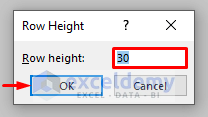
Fit Text by Changing Row Height for Entire Excel Worksheet

Upon pressing OK, you will get the below output. We can see that the height of all rows in the worksheet is adjusted to 30. The text of rows, 5 and 9 are also fully visible now.

Things to Remember

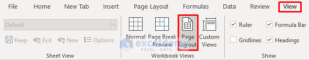
In Excel, there are different row height units. You can adjust row height in inches, centimeters, or millimeters. Go to View > Page Layout. Select a row >> right-click on it >> select Row Height from the context menu. You can use a specific unit in that box.

Things to Remember

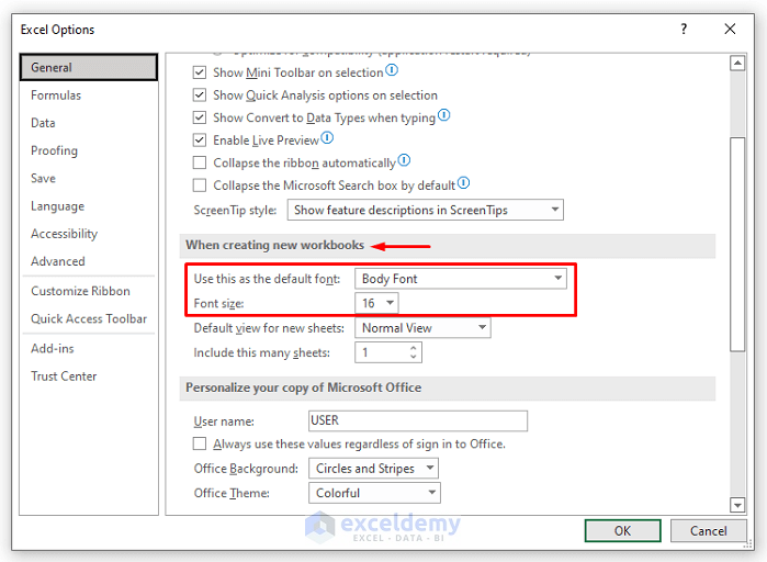
In Excel, you can change and restore the default row height too. Go to File > Options > General. Change the Font Size from the When creating new Workbooks. This change will only be applied when you restart the excel and create a new workbook.