How to Add Watermark in Excel (2 Easy Ways)

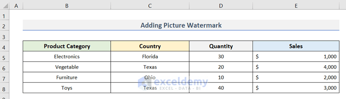
We’ve used an Excel workbook with multiple worksheets that contain the same dataset. The dataset contains the Categories, Countries, Quantities, and Sales of different Products.

Method 1 – Add Watermark by Using the Excel Ribbon

Case 1.1 – Picture Watermark

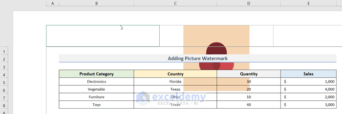
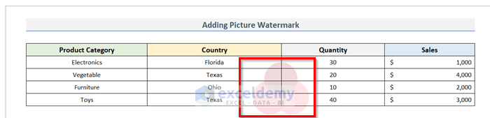
We have a dataset (B4:E8) of an Excel worksheet like the screenshot below. We have to add a picture watermark to it.

Steps:

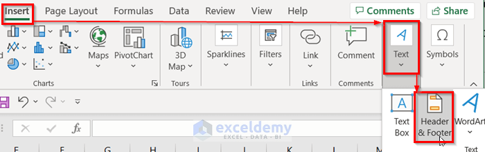
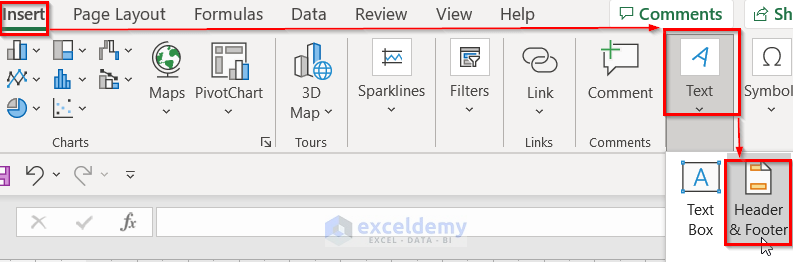
• Go to the Insert tab and click on the Text option.
• Click the Header & Footer option from the drop-down.

• A Header section will appear with a blinking cursor in the middle section of the sheet. We have to insert the picture here.

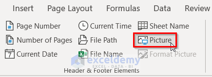
• Click on the Picture to add the desired image from the Header & Footer option.

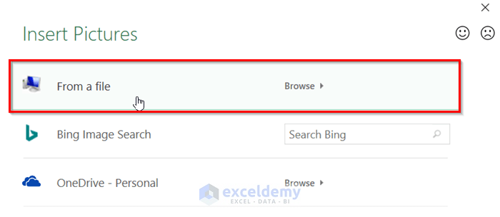
• A window will appear which has three options of inserting a picture.
• We chose the From a File option to upload the picture that is already available on our computer. We can also insert pictures online by using the other two options.

• Notice a &[Picture] entry inside the header cell similar to the image below.

• After clicking on any portion of the document outside the header area, the watermark image becomes visible.

Recolor the Watermark

We want to gray out the watermark picture.

Steps:

• Go to the Insert tab and select the Text option.
• Click Header & Footer.

• A Header and Footer tab will open in the Ribbon area.
• Select Format picture.

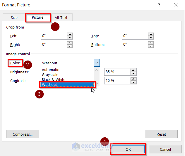
• A Format Picture window will appear.
• Select Picture, then go to the Color drop-down.
• Select Washout and hit OK

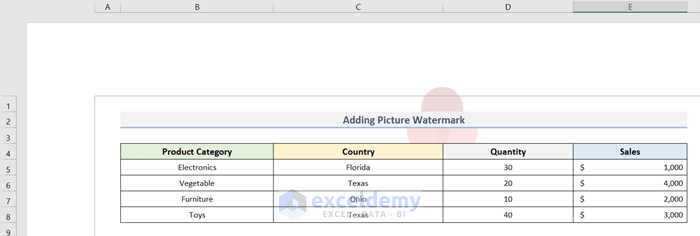
• We will see the washed-out watermark in the background.

Reposition the Watermark

Steps:

• Go to Insert, then to Text, and choose Header & Footer.

• The Header section will open.
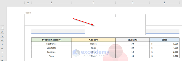
• If we want to push the picture downward, we need to add some blank lines before the code &[Picture]. To enter blank lines, we need to place the cursor at the beginning of the code and hit Enter.
• If you want to show the watermark at the center of the page, enter enough line breaks to push it down to the center.

• We can see that our watermark picture is positioned in the center.

Resize the Watermark

Steps:

• Go to Insert.
• Select the Text drop-down.
• Choose Header & Footer.

• Select Format Picture from the Header & Footer tab.

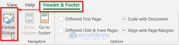
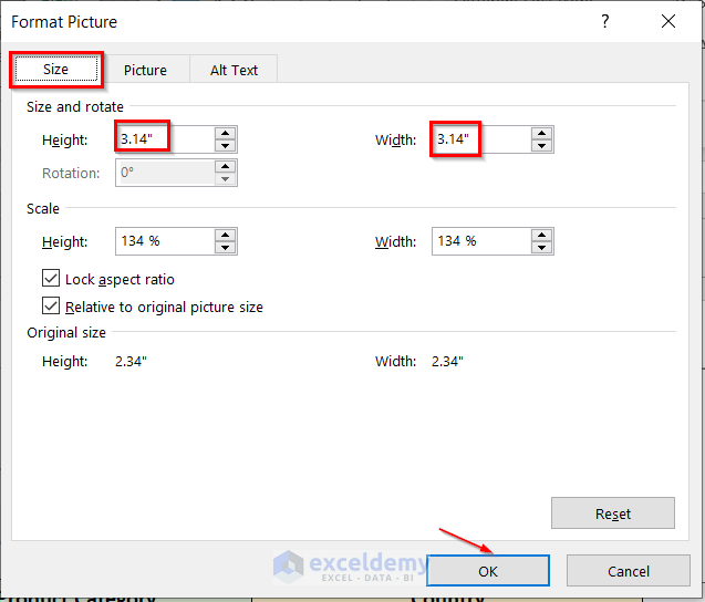
• A Format Picture dialogue box will appear.
• Go to Size. We can change the height and width of the watermark here.
• Click the OK button.

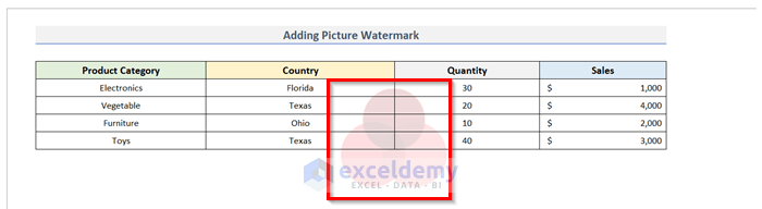
• We have increased the height and width of the watermark.

• We can see the result below.

Read More: How to Fix Watermark in Excel

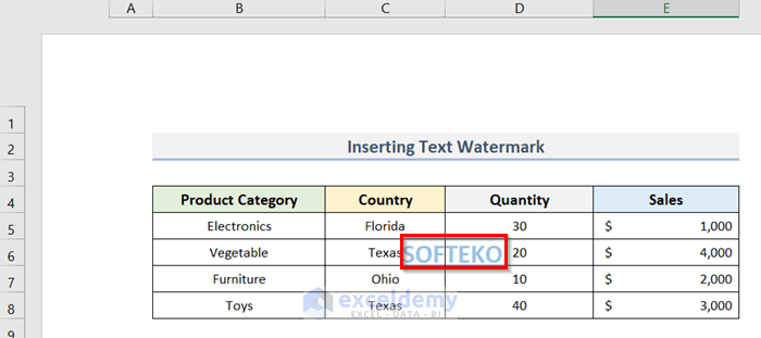
Case 1.2 – Text Watermark

Steps:

• Select Insert, then choose Text and click Header & Footer.

• Enter the watermark text where you can see the blinking cursor in the header section.

• After entering the watermark text, increase its font size by selecting it.

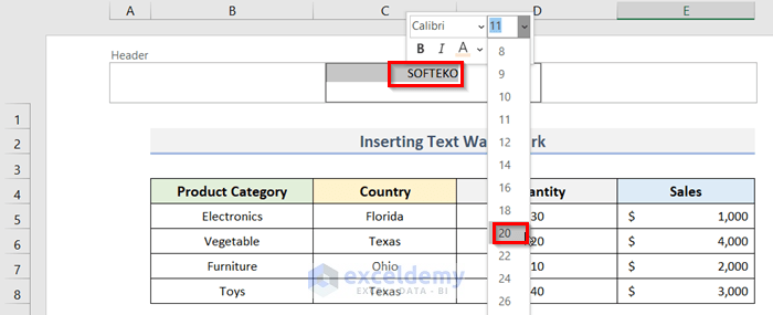
• The font size of the watermark text has increased.

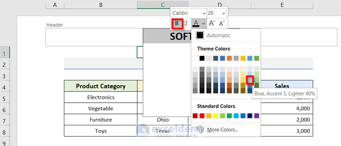
• We can change the color of the watermark text by selecting it.

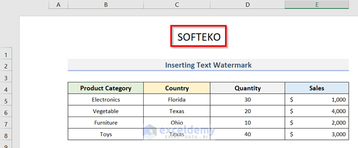
• We can change the position of the watermark by keeping the cursor in front of the text and hitting the Enter button.

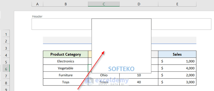
• Here’s the result.

Method 2 – Insert a Watermark in Excel with the WordArt Feature

Steps:

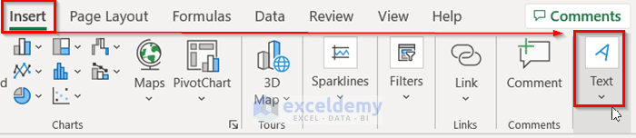
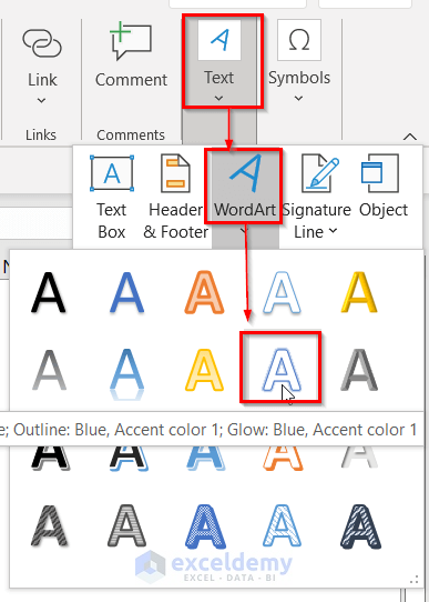
• Go to the Insert tab and click on Text

• Click on WordArt and select a style.

• Enter the watermark text into Your text here.

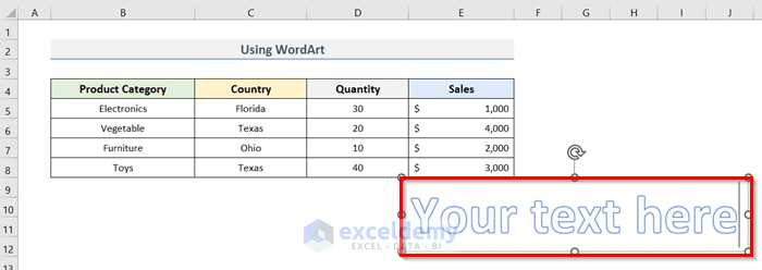
• Click on any cell outside the box to set the watermark.

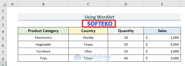
• We can format the text watermark by selecting it.
• Our formatted text watermark looks like the picture below.

Read More: How to Move Watermark in Excel

How to Remove a Watermark in Excel

Steps:

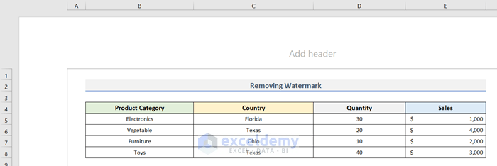
• We can see a picture watermark on an Excel dataset.

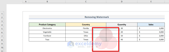
• Click on the header area of the spreadsheet. This will make the watermark active.

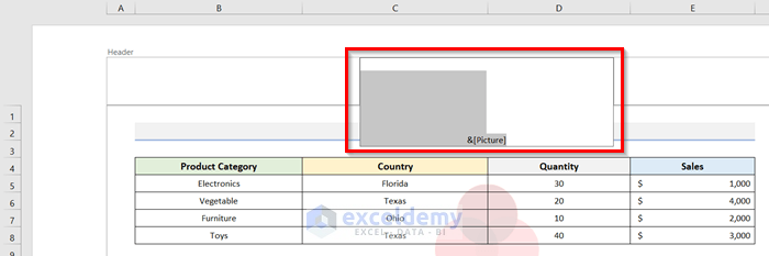
• Press the Delete or Backspace key on the keyboard. This will remove the watermark.

• Here’s the result.

Read More: How to Remove Page 1 Watermark in Excel

Download the Practice Workbook

<< Go Back to Watermark | Page Setup | Print in Excel | Learn Excel