What Is Accrued Vacation Time?
Generally, employees get a certain amount of days to leave for vacation, personal reasons, or sickness. But if the employee hasn’t used the earned leave days then this will be called Accrued Vacation Time. And the employee will earn the amount equivalent to the accrued vacation time at the end of the year. This is also called PTO – Paid Time Off.
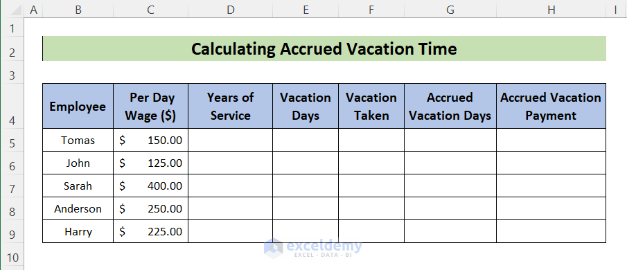
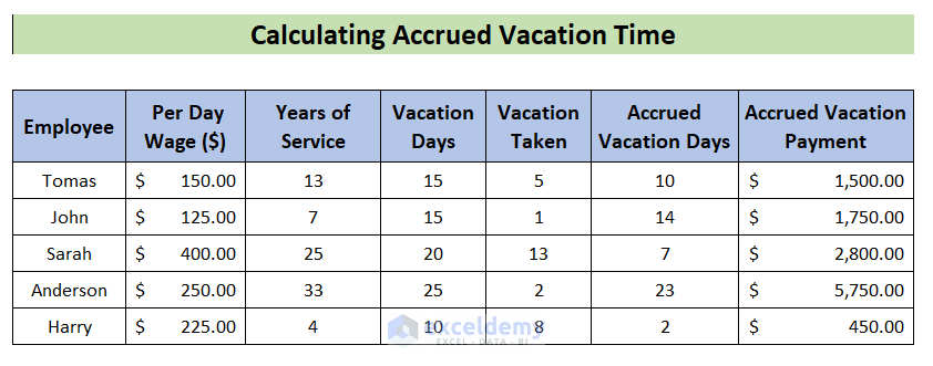
The sample dataset has details for a number of employees including their wage, years of service, and vacations taken.
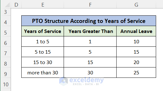
Step 1 – Create Paid Time Off (PTO) Structure
- Create a table with the relevant information regarding paid leave days for employees based on their years of service.
- Create one more column that will be used for the VLOOKUP formula.
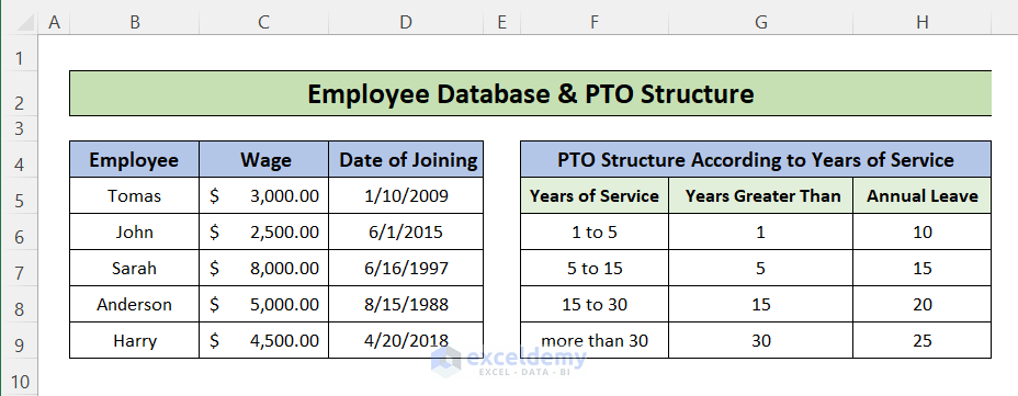
Step 2 – Create Employee Database with Joining Dates
Collect the data of employee names, joining dates, and wages and make a table with this data in an Excel worksheet.
Step 3 – Calculate Years of Service
Use the DATEDIF function to calculate the years from the joining date until today. Enter this formula into cell D5:
=DATEDIF(Database!D5,NOW(),"Y")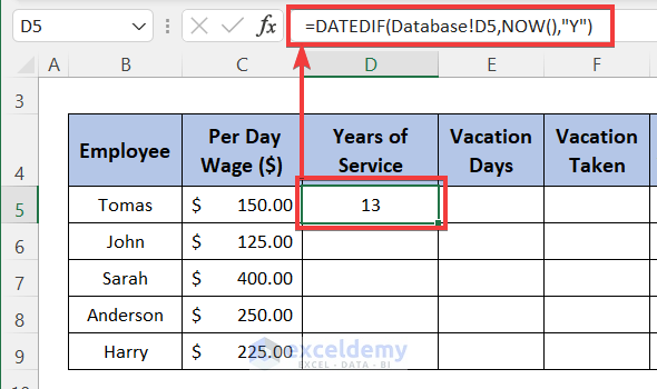
- Drag the Fill Handle icon to paste the formula to the other cells in the column.
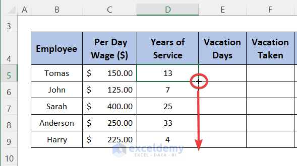
Step 4 – Calculate Allowed Vacation Days
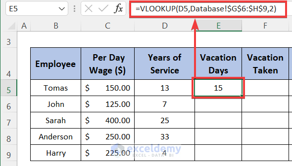
Enter the VLOOKUP formula into the cell E5:
=VLOOKUP(D5,Database!$G$6:$H$9,2)Formula Explanation
- Lookup_value = D5
The function will look for the value in cell D5 in the lookup table. - Table_array = Database!$G$6:$H$9
The range of cells that the function will search for the lookup value. - Col_index_num = 2
It will return the value of column 2 in the lookup table from the row where the lookup value exists.
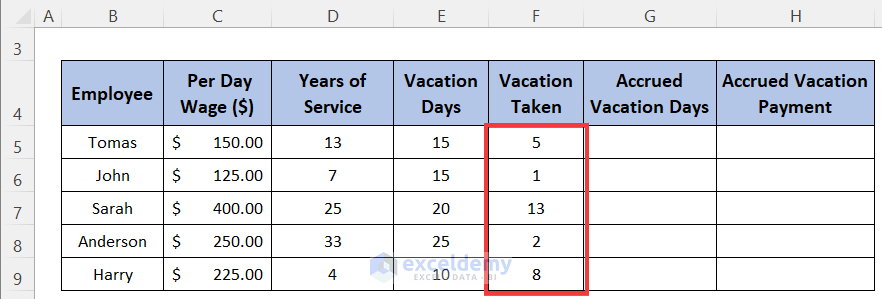
Step 5 – Insert the Number of Vacation Days Taken from Employees’ Attendance Tracker
Open the Employee attendance tracker for that year and link the cell containing the total leave days in cell F5 or insert the values manually in the vacation taken column.
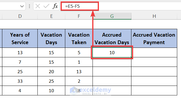
Final Step – Calculate Accrued Vacation Time
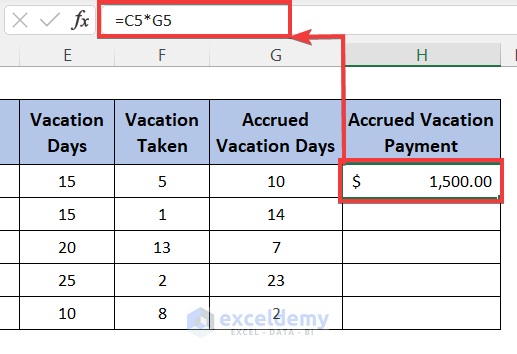
Calculate the accrued vacation days with this formula:
You can calculate the accrual vacation payment to encash the leave days not taken. Enter the formula:
The accrued vacation days and the accrued vacation payments of the employees of the company have been calculated.
Calculate Accrued Vacation Time in Excel Excluding Probationary Period
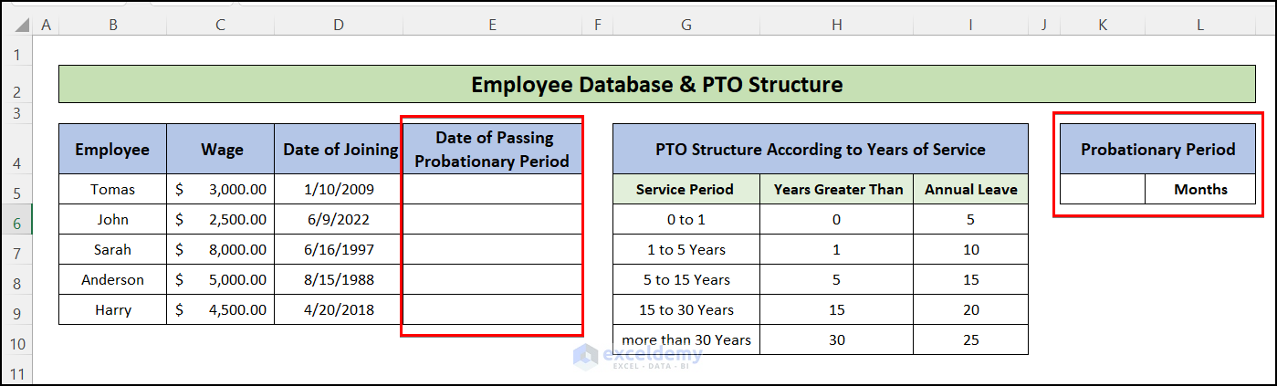
- Insert a new column to calculate the date the probationary period ended (or passed). Select a cell to record the length of the probationary period in months.
- Insert the following formula into cell E5 and drag the fill handle to the last row of the table
=EDATE(D5,$K$5)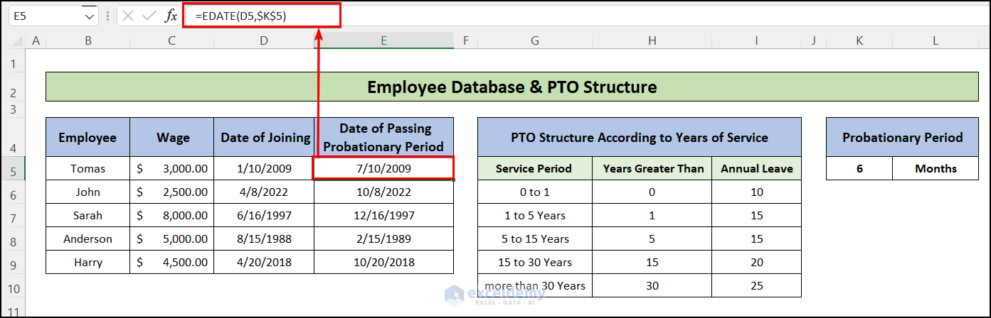
- Go to the Accrued Vacation worksheet and rename column D as Months of Service. Add a new column after that named Years of Service.
- Insert the following formula into the cell D5:
=IFERROR(DATEDIF(Database!E5,NOW(),"M"),"In Probation")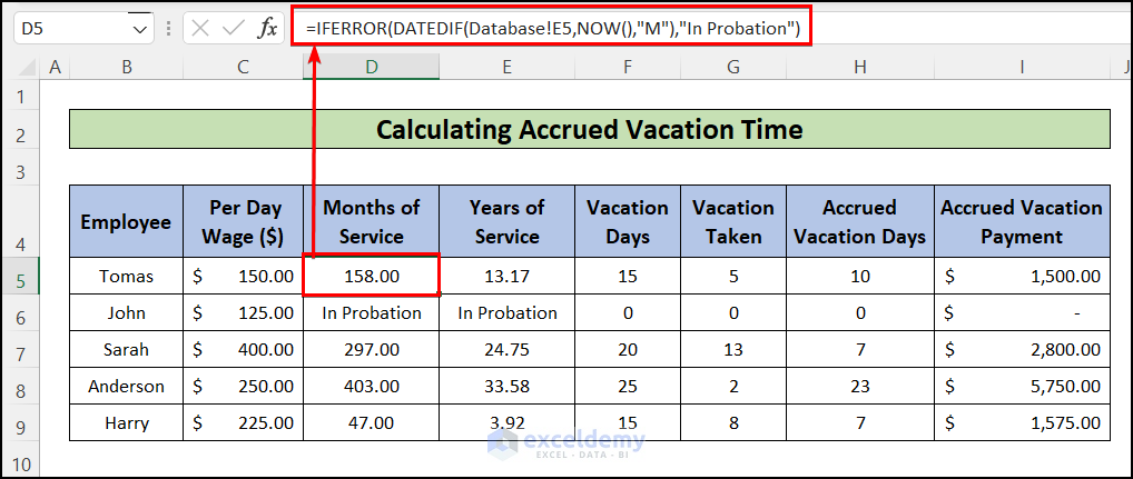
- Calculate the years of service using the following formula in cell E5 and drag the fill handle to apply similar formula for other cells also.
=IFERROR(D5/12,"In Probation")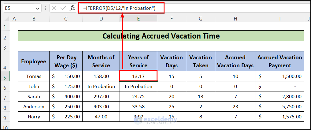
- Insert the following formula to get the allowed accrued vacation time for the employees in cell F5:
=IFERROR(VLOOKUP(E5,Database!$H$6:$I$10,2),0)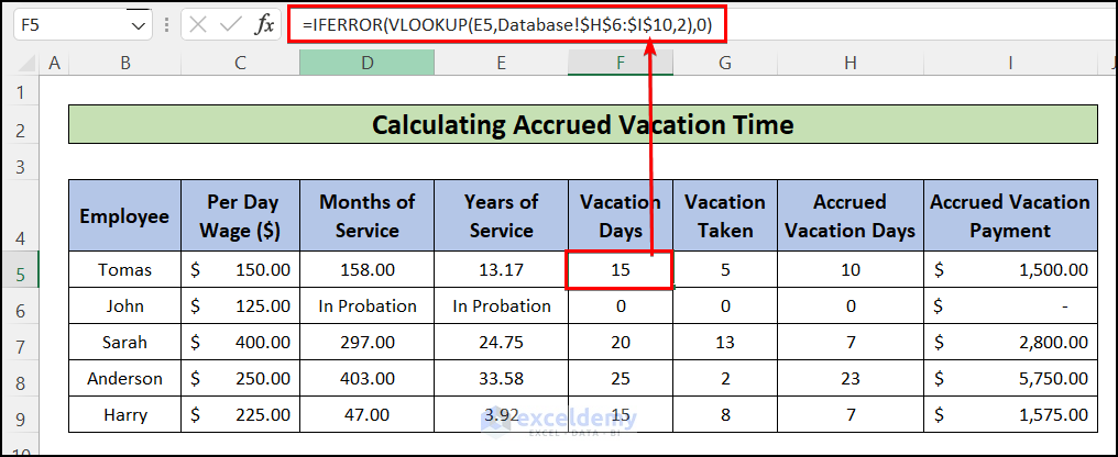
- Calculate the remaining part using the Final Step of the previous method.
Download Practice Workbook
You can download the practice workbook from here:
<< Go Back to Leave Calculation | Formula List | Learn Excel
Get FREE Advanced Excel Exercises with Solutions!

I have a question.. How can you figure in a 60 day probationary period? Our employees don’t start accruing time until they’ve completed a 60 day probation.
Thanks!
Hello BRYAN!
As per your question, I have added a new portion in the article which contains the method how you can calculate the accrued time after the completion of probationary period automatically.
I hope, your problem will be solved in this way. You can share more problems in an email at [email protected]