How to Split Column in Excel Power Query (5 Easy Methods)

While working with large Microsoft Excel, sometimes we need to split columns using a power query. Splitting columns by using the power query is an easy task. This is a time-saving task also. Today, in this article, we’ll learn five quick and suitable ways to split column in Excel power query effectively with appropriate illustrations.

Let’s assume we have an Excel large worksheet that contains the information about several sales representatives of Armani Group. The name of the sales representatives, the Product Name, and the Revenue Earned by the sales representatives are given in Columns B, C, and D respectively. We can easily split a column using the Power Query Editor in Excel by using the Delimiter command, Positions command, and so on. Here’s an overview of the dataset for today’s task.

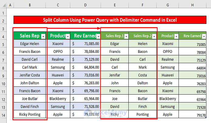
1. Using Delimiter Command to Split Column in Excel Using Power Query

In this method, we will split a column by using the Power Query Editor with the Delimiter command. This is an easy task and time-saving also. To do that, you have to take your data in Power Query Editor first. Then you will be able to split a column using the power query. Let’s follow the instructions below to split a column using the Power Query in Excel!

Step 1:

• First of all, select your entire data range from your dataset. We select B4:D14 and then press Ctrl + T simultaneously on your keyboard. After that, instantly a dialog box named Create Table will appear in front of you. From that dialog box, press OK.

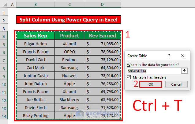
• As a result, you will be able to create a table. After that, from your Data tab, go to,

Data → Get & Transform Data → From Table /Range

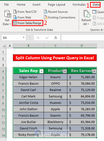
• Hence, you will be taken to the Power Query Editor.

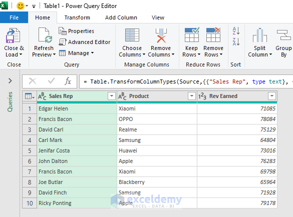
Step 2:

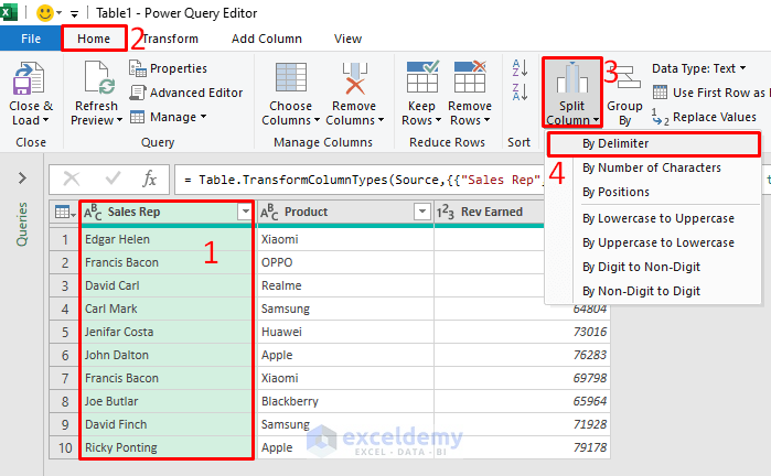
• Now, From the Power Query Editor, firstly select the column with the heading Sales Rep. After that, from the Home tab, go to,

Home → Transform → Split Column → By Delimiter

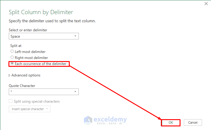
• As a result, a Split Column by Delimiter dialog box will appear in front of you. From that dialog box, select Each occurrence of the delimiter under the Split at At last, press OK.

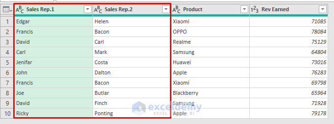
• After completing the above process you will be able to split a column named Sales Rep with the Power Query Editor which has been given in the below screenshot.

Step 3:

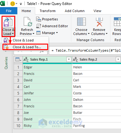
• Now, select Close & Load → Close & Load To as shown in the following picture.

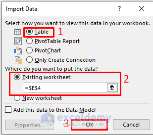
• Hence, a dialog box named Import Data pops up. From the Import Data dialog box, firstly, select the Table option under the Select how you want to view this data in your workbook Secondly, type =$E$4 in the Existing workbook typing box. At last, press OK.

• After completing the above process, you will be able to import data in your Excel sheet from the Power Query Editor which has been given in the below screenshot.

Read More: How to Split One Column into Multiple Columns in Excel

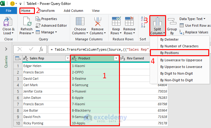
2. Applying Positions Command to Split Column with Excel Power Query

Now, we will split a column by using the Power Query with the Positions command. We will split a column with the position of the text. This is an easy task and time-saving also. Let’s follow the instructions below to split a column using the Power Query Editor in Excel!

Steps:

• First of all, select a column named Product, and then from the Home tab, go to,

Home → Transform → Split Column → By Positions

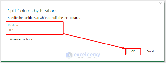
• As a result, a Split Column by Positions dialog box will appear in front of you. From that dialog box, firstly, type 0,2 in the typing box named Positions. At last, press OK.

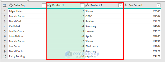
• After completing the above process you will be able to split a column named Product with the Power Query Editor which has been given in the below screenshot.

Read More: How to Split Column in Excel by Comma (8 Quick Methods)

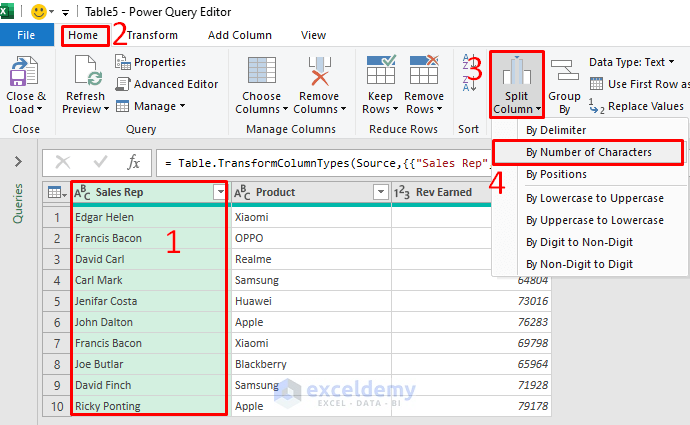
3. Performing Number of Characters Command to Split Column Using Power Query

In this method, we will split a column by using the Power Query with the Number of Characters command. We will split a column with the number of characters in the text. This is an easy task and time-saving also. Let’s follow the instructions below to split a column using the Power Query Editor in Excel!

Step 1:

• First of all, select a column named Product, and then from the Home tab, go to,

Home → Transform → Split Column → By Number of Characters

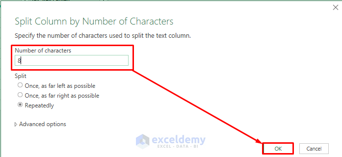
• As a result, a Split Column by Positions dialog box will appear in front of you. From that dialog box, firstly, type 8 in the typing box named Positions. At last, press OK.

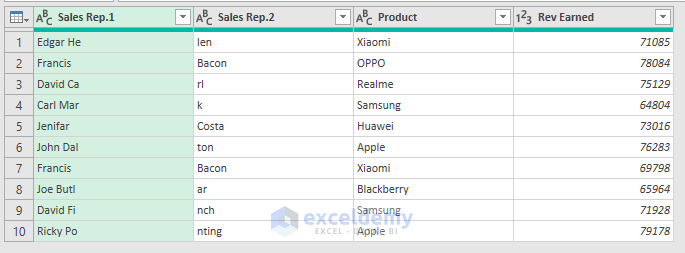
• After completing the above process you will be able to split a column named Product with the Power Query Editor which has been given in the below screenshot.

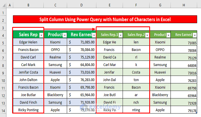
Step 2:

• To import the split column in the Excel sheet, simply repeat Step 3 of method 1.

Read More: How to Split Column by First Space in Excel (with Easy Steps)

4. Applying Uppercase to Lowercase Command to Split Column in Power Query

In this method, we will split a column by using the Power Query with the Uppercase to Lowercase command. We will split a column from the uppercase to lowercase in the text. This is an easy task and time-saving also. Let’s follow the instructions below to split a column using the Power Query Editor in Excel!

Step 1:

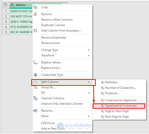
• First of all, select a column named Address. Now, press right-click on your mouse. Hence, a window pops up. From that window, go to,

Split Column → By Uppercase to Lowercase

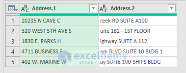
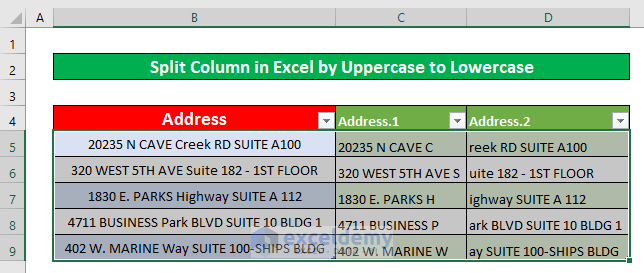
• Further, you will be able to split the column named Address by Uppercase to Lowercase.

Step 2:

• To import the split column in the Excel sheet, simply repeat Step 3 of method 1.

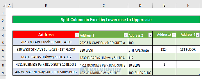
• You can also split a column by the column named Address by Lowercase to Uppercase.

Read More: Split Column in Excel by Word (5 Effective Ways)

5. Using Digit to Non-Digit Command to Split Column Using Power Query

Last but not the least, we will split a column by using the Power Query with the Digit to Non-Digit command. We will split a column from the digit to the non-digit in the text. This is an easy task and time-saving also. Let’s follow the instructions below to split a column using the Power Query Editor in Excel!

Step 1:

• First of all, select a column named Address. Now, press right-click on your mouse. Hence, a window pops up. From that window, go to,

Split Column → By Digit to Non-Digit

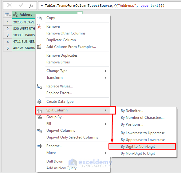
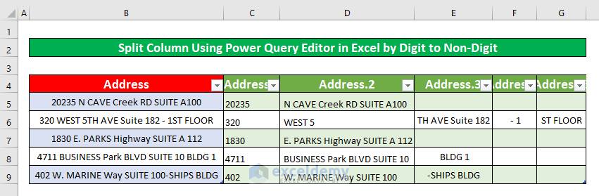
• Further, you will be able to split the column named Address by Digit to Non-digit.

Step 2:

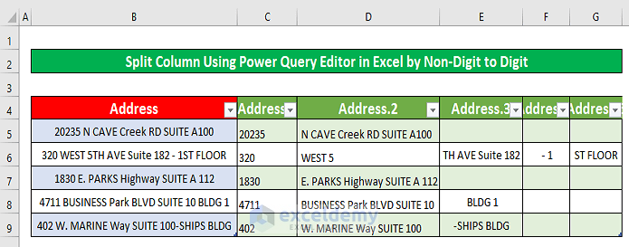
• To import the split column in the Excel sheet, simply repeat Step 3 of method 1.

• You can also split a column by the column named Address by Non-digit to Digit.

Read More: How to Split One Column into Multiple Columns in Excel Formula

Things to Remember

➜ While a value can not found in the referenced cell, the #N/A error happens in Excel.

➜ You can press Ctrl + T simultaneously on your keyboard to create a table.

Download Practice Workbook

Download this practice workbook to exercise while you are reading this article.

Conclusion

I hope all of the suitable methods mentioned above to split columns using power query will now provoke you to apply them in your Excel spreadsheets with more productivity. You are most welcome to feel free to comment if you have any questions or queries.

Related Articles

• Split Date and Time Column in Excel (7 Easy Methods)