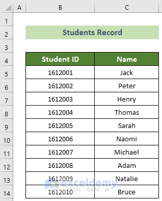
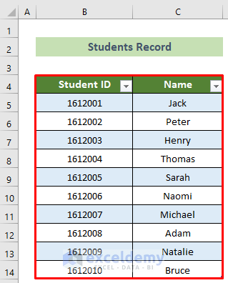
There’s a dataset showcasing students’ IDs and names,
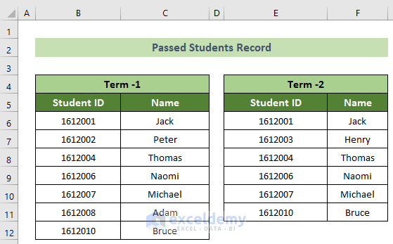
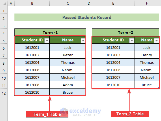
and another one containing the Passed Students’ Records in Term 1 and Term 2.
To find the students who passed in both terms and those who passed only in one term:
Example 1 – Comparing Two Tables and Merging All Values
Find the students who passed in one term only:
Steps:
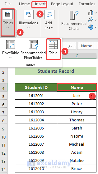
- Convert the datasets into tables.
- Click any cell in the Students Record range >> go to Insert >> Tables >> Table.
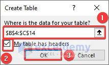
- In the Create Table window, enter B4:C14 >> check My table has headers >> click OK.
- Students Record is converted into a table.
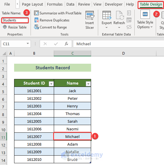
- To name the table, click any value inside the table >> go to Table Design >> enter Students in Table Name:.
- Create two other tables: Term_1 and Term_2.
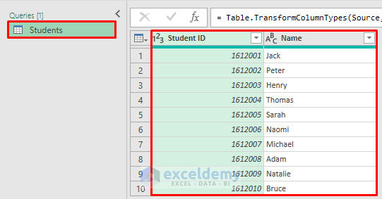
- Go to the Power Query window, right-click any cell inside the Students Record table and choose Get Data from Table/Range.
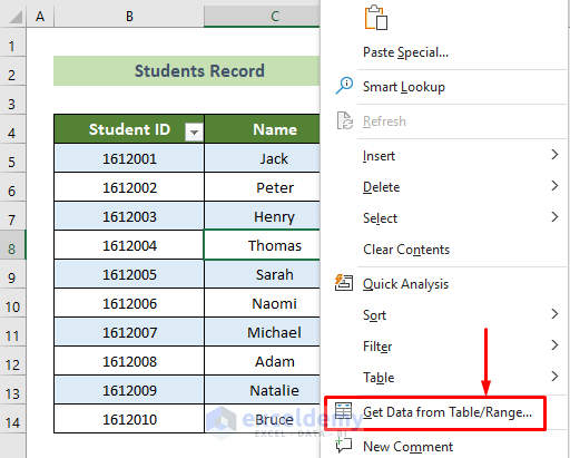
The Students table is displayed in the Power Query.
- In the Home tab of the Power Query, click Close & Load >> choose Close & Load To…
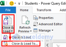
- In the Import Data window, select Only Create Connection and click OK.
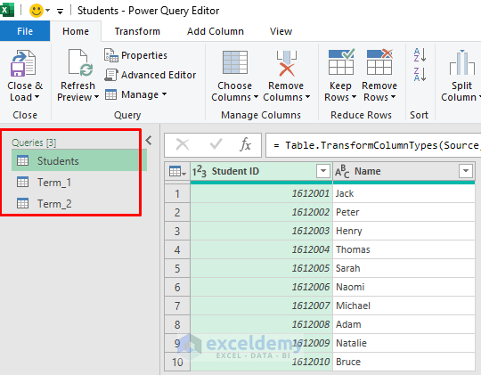
- Repeat the previous procedure for the Term_1 and Term_2 tables to import data to the Power Query.
- Right-click the Queries pane >> choose New Query >> Other Sources>> Blank Query.
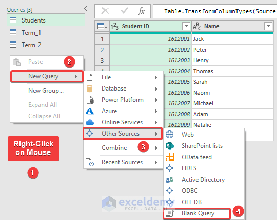
- A new query will be created.
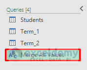
- Name it “Merge All Values”.
- Click the Merge All Values query and enter the following formula to compare the two tables and merge values.
=List.Union({Term_1[Name],Term_2[Name]},Comparer.OrdinalIgnoreCase)- Press Enter.
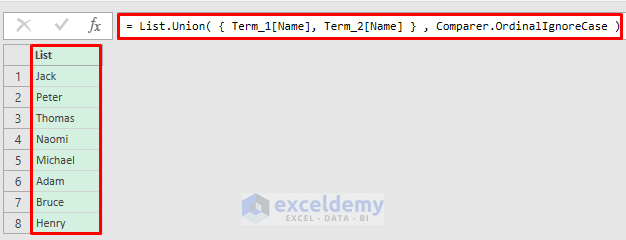
You have compared and merged the two tables and found the students who passed in one term.
- To get the IDs, go to Query Settings >> APPLIED STEPS >> right-click Source >> choose Insert Step After.
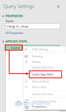
- A new step will be added.
- Name it “Insert IDs”.
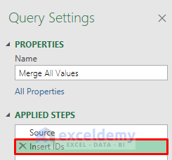
- Click the Insert IDs step and enter the following formula in the formula bar.
=Table.SelectRows(Students,eachList.ContainsAny({[Name]},Source))- Press Enter.
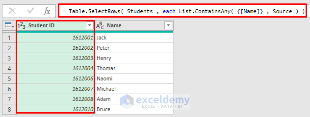
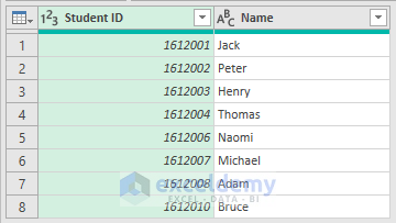
You will see the students’ IDs.
You have compared and merged the two tables.
This is the final output.
Example 2 – Comparing Two Tables with the Power Query and Finding the Common Values
To find the students who passed in both terms:
Steps:
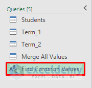
- Follow the first 16 procedures in Example 1 to prepare tables for the power query and create a new query: “Find Common Values”.
- Click Find Common Values and enter the following formula in the formula bar.
=List.Intersect({Term_1[Name],Term_2[Name]},Comparer.OrdinalIgnoreCase )- Press Enter.
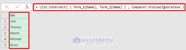
- You find the students who passed in both terms.
- To add their IDs, go to Query Settings >> APPLIED STEPS >> right-click Source >> choose Insert Step After.
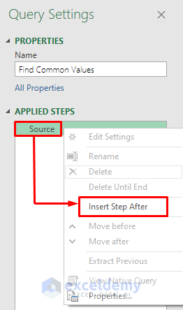
- A new step is created.
- Name it “Insert IDs”.
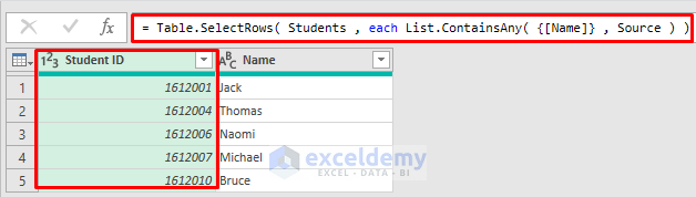
- Click the Insert Ids step >> enter the following formula in the formula bar >> press Enter.
=Table.SelectRows(Students,each List.ContainsAny({[Name]},Source))- Students’ IDs are imported.
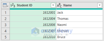
This is the output.
Download Practice Workbook
Download the practice workbook here.
Related Articles
<< Go Back to Power Query Excel | Learn Excel
Get FREE Advanced Excel Exercises with Solutions!
