Method 1 – Using the ‘Data Analysis’ Tool
Step 1: Download and Install the Data Analysis ToolPak
- Go to the top left corner of Excel and click on the File tab.

- Click on Option, which is the below left on the file.
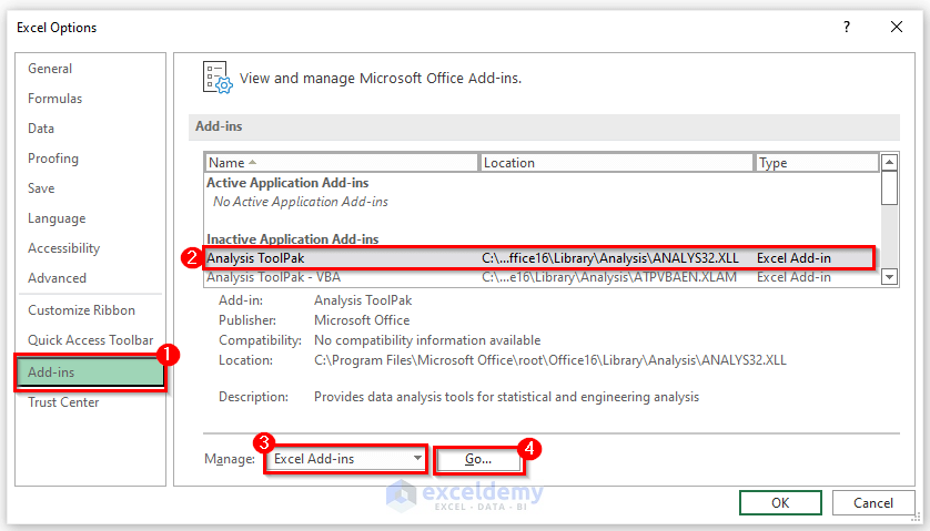
- The Excel Options menu will appear. Click on the Add-ins option and pick Analysis Toolpak.
- On the Manage drop-down menu bar, choose Excel Add-ins.
- Click Go.
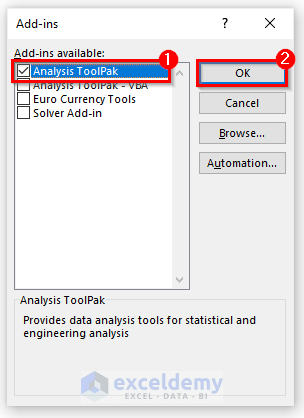
- The Add-ins pop-up window will appear.
- Check the Analysis ToolPak under the Add-ins available check box.
- Click on the OK button to enable the Data Analysis menu.
- As indicated above, the ‘Data Analysis’ menu should appear in the Data tab.

Note: In Excel for Mac, the Analysis ToolPak is no longer available. You’ll need to download a third-party analytic tool to do some different measures.
Step 2: Evaluate Two-Sample T-Test Statistics
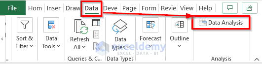
- Go to the Data tab from the ribbon.
- Click on Data Analysis under the Analysis group.
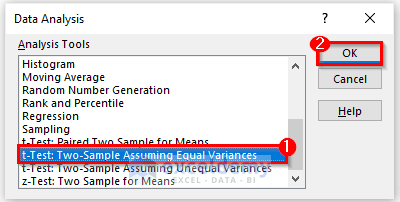
- This will open the Data Analysis dialog box.
- Scroll down to the dialog and find the t-test options.
- Select t-test: Two-Sample Assuming Equal Variances.
- Click OK.
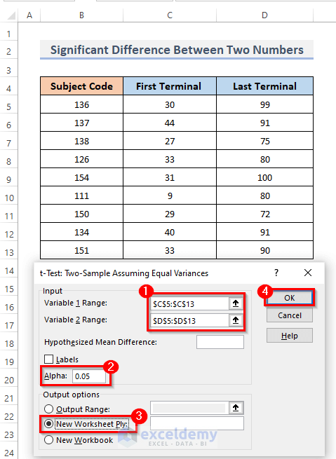
- Fill the cells with your data.
- Pick the Variable 1 Range box in the Input option.
- Select the column holding the data for the First Terminal. When you choose cells in our worksheet, the range should be displayed in the box.
- Repeat the procedure for Variable 2 Range and any other data column in the Last Terminal. We can adjust the output settings and alpha value if necessary, although the default alpha 0.05 is generally sufficient.
- Select the Output options, New Worksheet Ply.
- Click OK.
The results of our statistical test will now be visible.
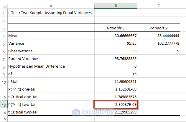
This will show the result of the t-test: Two-Sample Assuming Equal Variances in another worksheet.
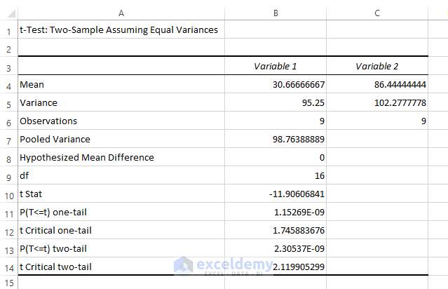
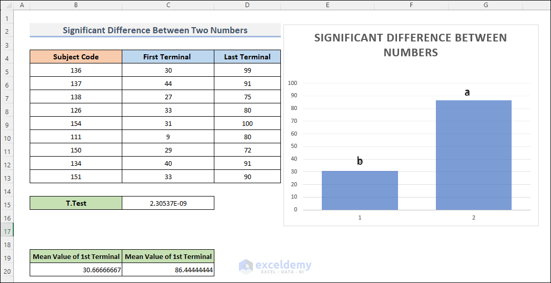
Final Result of Significant Difference
In cell B13, the P(T = t) two-tail is less than the alpha value of 0.05. We can conclude that the means of our two trials differ by a statistically significant amount, and we can say the difference is significant.
Note: T-tests are resilient to discrepancies among variances when both categories have an equal or approximately equivalent number of instances and standard portion size. If one group’s variance is double that of others, it’s reason to be concerned! Minor deviations, on the other hand, are unimportant.
Use the uneven variances variant of the 2-sample t-test if you already have differences with regard and a different number of respondents.
Method 2 – Using a Formula to Get Significant Difference Between Two Numbers
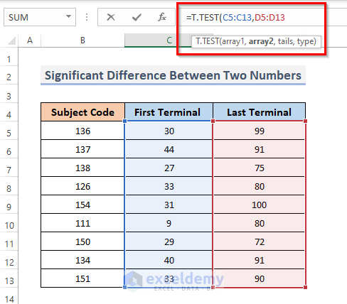
Step 1: Select the Range
- Enter the following formula into a cell:
=T.TEST(array1, array2,tails,type)- The first set of data is referred to as array1, while the second set of data is array2.
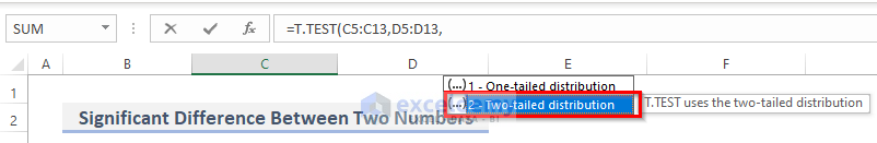
Step 2: Choose the Tailed Distribution
- The type pertains to whether you want to operate a one- or two-tailed test. In the instance at left, we input the second option, which implies a two-tailed test;
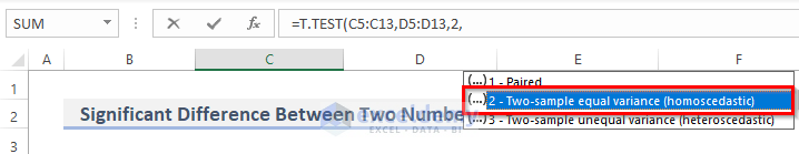
Step 3: Choose a Type of T-Test
- Select the t-test type. We will input the option, as shown in the use of each type of t-test in the first method.
- Select the number 2 option because it’s the Two-sample equal variance.
Final Result of Significant Difference
Click on the resulting cell, we will see the formula for the t-test in the formula bar.
=T.TEST(C5:C13,D5:D13,2,2)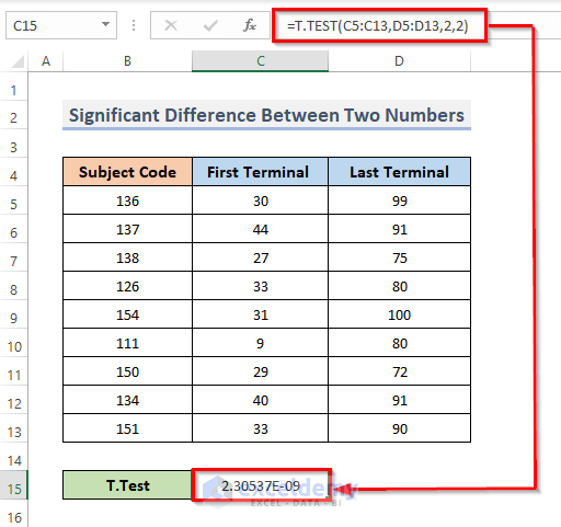
Note: The t-test determines the likelihood that the difference in the two values is due to randomness. It is common practice to declare that if the probability is less than 0.05, the difference is significant,’ indicating that it is not due to chance.
Read More: How to Calculate Significant Difference Between Two Means in Excel
Download the Practice Workbook
You can download the workbook and practice.
<< Go Back to Excel for Statistics | Learn Excel
Get FREE Advanced Excel Exercises with Solutions!

Good day
This has been helpful.
However, I am not from a statistic background I am an agronomist and normally just outsource.
I would like to find out how I can then use this significant value in drawing my graphs.
For instance, the mean values are made clear by the ANOVA and I can easily pick them and draw my graph showing the various means from my treatments. Now I would like to put asterisks on graphs to show which one did better than the other and which did poorly.
Can I then just look at the largest mean then put an “a” asterisk on top of the bar, then subtract the TTest value and find which treatment (I have 4 treatments) mean is closest then denote it with a “b” and so forth until my treatments are all covered?
Please I have minimal background in stats.
Regard
Hello OLWETU,
I hope you are doing well. Well, thank you for your query. Adding asterisks to graphs is a significant way to show the difference between two or more groups. You can get the mean value of the treatments using the ANOVA method. Then plot the mean values in the graph. This part is relatively easy and already shown in the article. Now, if you want to add the asterisks to the chart to define the largest mean then select the chart and check the Data levels as below.
Therefore, write down “a” in a cell and double-click the value of the highest mean value. Once you click on the data levels you will see the options of selecting data levels. Finally, select Choose Cell to get the asterisks as “a”.
Now, apply the MIN function to get the minimum value of the mean values and inter asterisks as “b” using the same process.