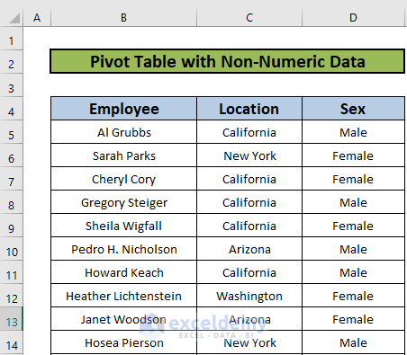
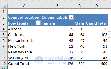
The following figure shows a table and a pivot table created from the table. The table has no numeric data, containing a list of some employees, their location, and gender. Though the table has no numeric values, it is possible to create a useful pivot table by counting the items.
Step 1 – Creating a Pivot Table from Text Data
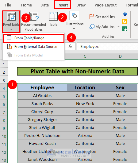
- Select the data range.
- Go to the Insert tab.
- Select PivotTable.
- Choose From Table/Range.
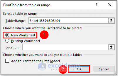
- A box will appear. Select New Worksheet to create a pivot table in a separate worksheet.
- Press OK.
- Excel will create a new pivot table.

Step 2 – Dragging Columns to PivotTable Fields
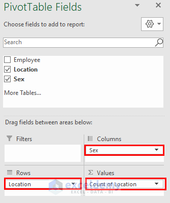
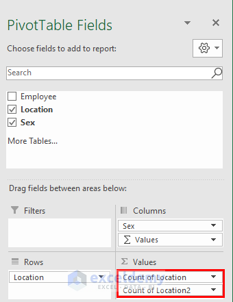
- Drag the Sex column to the Columns field.
- Drag the Location column to the Rows field and Values field.
- Excel will automatically show the Count of Location when you drag the Location column to Values Field.
- Excel will return the following output.
How to Use a Pivot Table to Show Non-Numeric Values as a Percentage
- Drag the Location column to the Values field.
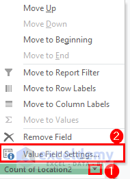
- Select the drop-down icon next to the new result you got.
- Select Value Field Settings.
- A Value Field Settings box will appear. Go to Show Values As.
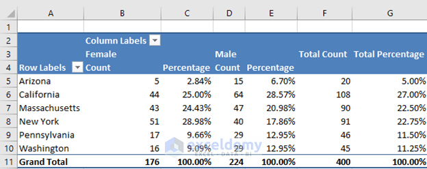
- Choose % of Column Total.
- Click OK.

- Excel will show the count of locations as a percentage as well in the output now.
Read More: How to Calculate Median in Excel Pivot Table
Download Practice Workbook
Download this workbook and practice while going through the article.
<< Go Back to Pivot Table Value Field Settings | Pivot Table in Excel | Learn Excel
Get FREE Advanced Excel Exercises with Solutions!

Is there a way we can compare 2 pivot tables with similar information to spit out the difference betwen the two ?
Hi there!
You can use the GETPIVOTDATA function to do that. Find out more in the following articles.
https://www.exceldemy.com/compare-two-pivot-tables-in-excel/
https://support.microsoft.com/en-us/office/getpivotdata-function-8c083b99-a922-4ca0-af5e-3af55960761f
Thanks for being with us.
Regards
Md. Shamim Reza (Exceldemy Team)
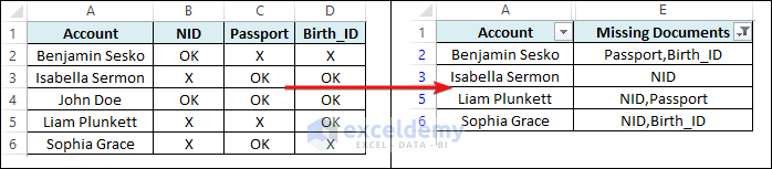
Hi, I just want to ask, I’m making a template for the company I am currently working (Bank here in the Philippines). I’m making a template to check if clients have submitted all necessary documents to open an account. I have made a table already. so in column a are list of sample accounts and for columns b onwards are for the required documents. i’ve made a drop down for those so we will only input either “ok” or x. is there a way i can summarize for example, account of john doe, all documents marked with x? thanks.
Hi there!
I am assuming that you want the following result.
Then follow the steps below.
First, apply the following formula in cell E2 and copy it down.
=TEXTJOIN(",",TRUE,IF(B2:D2="X",$B$1:$D$1,""))Then, filter out the blank cells from column E.
Next, hide columns B to D.
Now you can print the summary data.
Please let us know if this is what you needed. If not then tell us more about it so that we may help. And thank you for being with us.
Regards
Md. Shamim Reza (Exceldemy Team)