How to Show Zero Values in Excel Pivot Table (2 Quick Ways)

If you have blank cells in your dataset, they will also be represented as blank in your Pivot Table. Here are 2 quick methods to display “Zero” instead of blank values.

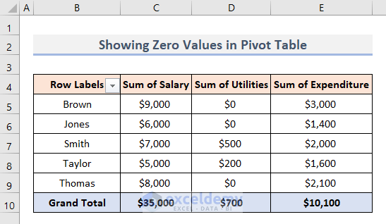
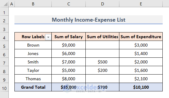
We’ll use the following sample Monthly Income-Expense List as a dataset to demonstrate the methods:

Method 1 – Use PivotTable Options

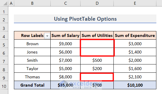
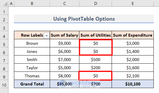
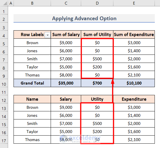
In the picture below, there are 3 blank cells, which were blank in the raw dataset, and therefore remained blank when converted into a Pivot Table. Let’s display those blank cells as $0 instead.

STEPS

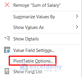
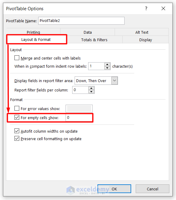
Right-click any cell in the pivot table and select PivotTable Options from the context menu.

Select Layout & Format in the Dialog box that opens.
In the Format section, insert 0 (zero) in the For empty cells show field.
Click OK.

The blanks will be replaced by zeroes in the pivot table.

Method 2 – Apply Excel Advanced Option

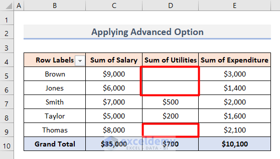
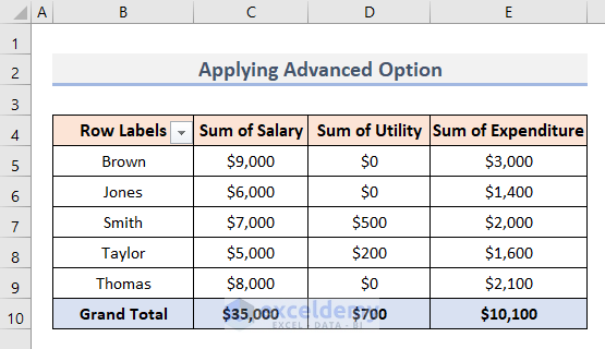
We will again display each blank cell in the pivot table as a $0.

STEPS

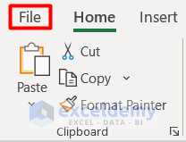
Click the File tab.

Click Options.

Select Advanced from the Options menu.
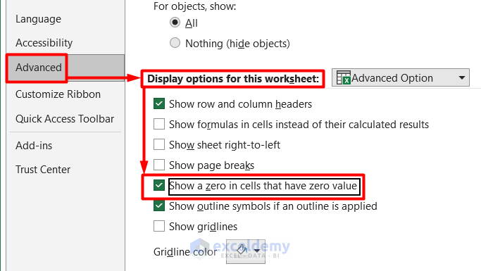
Select the Advanced option.
Under Display options for this worksheet, tick Show a zero in cells that have zero value.
Click OK.

Blank cells are filled with $0 in the pivot table.

Note: When using the Advanced option, you must have Zero (0) values in the original dataset, not blanks, to create Pivot Table values also displaying Zero (0).