Here’s a GIF overview of hiding zeroes or blank values from a pivot table.
Hide Zero Values in Pivot Table in Excel: 3 Easiest Ways
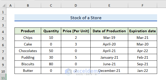
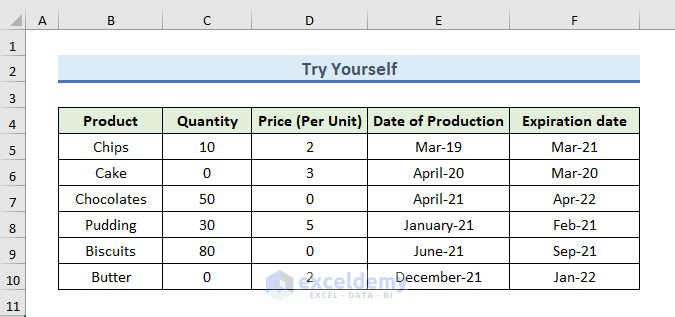
Here’s a dataset of a store’s stock, showing the quantities and prices of some products and their production and expiration dates. Note that some prices and quantities are empty. Let’s make a Pivot Table from the dataset.
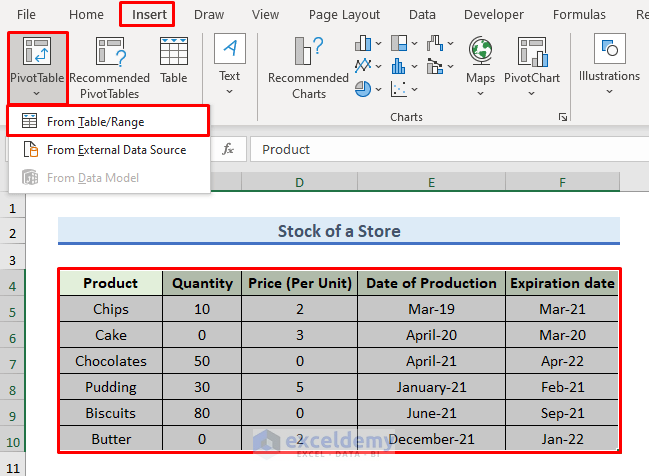
- Select the dataset.
- Click on Insert, choose Pivot Table, and select From Table/Range.
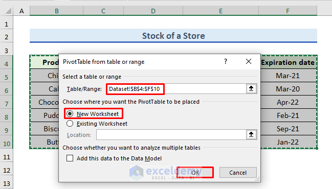
- A window named Pivot Table from table or range window will open. In the Table/Range field, you can automatically see the selected range.
- Tick New Worksheet and press OK.
- Excel will create the Pivot Table in a new worksheet.
- Click on the table, and in the right side of the sheet, select these 3 options: Products, Quantity, and Price (Per Unit).
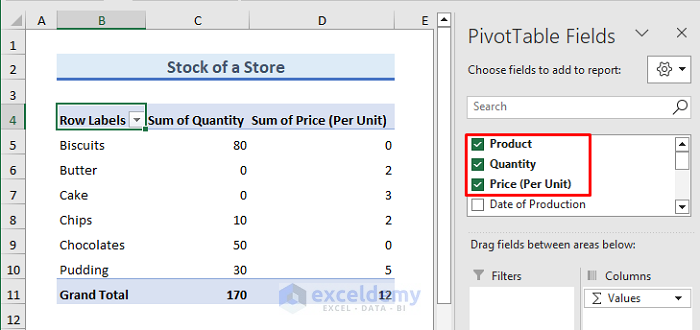
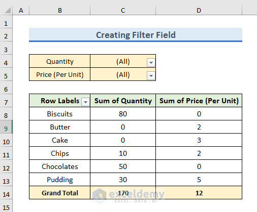
- Our Pivot Table is ready.
- Let’s hide the zero values.
Method 1 – Creating a Filter Field to Hide Zero Values in a Pivot Table
Steps:
- Click on the pivot table that you created from the dataset.
- On the right side, you will see PivotTable Fields.
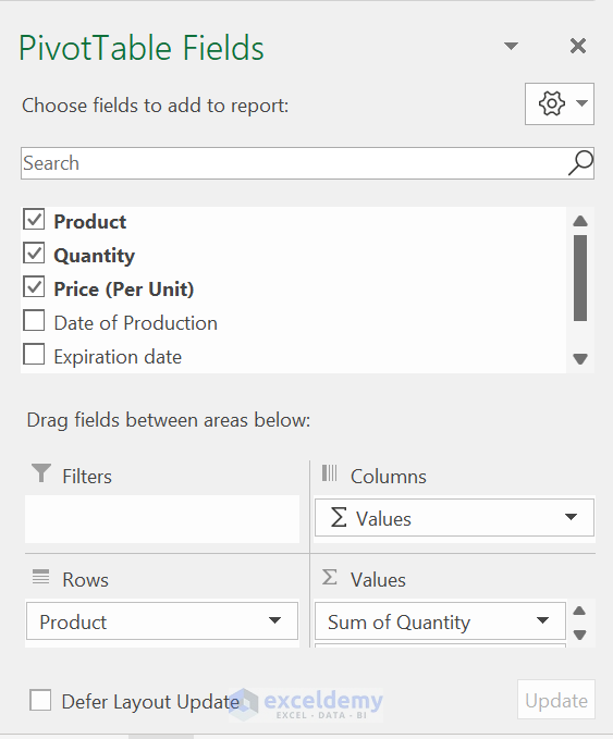
- From the pivot table fields, drag the Quantity into the Filter field.
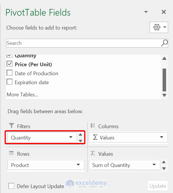
- Drag the Quantity into the Filter field.
- You will see two Filter options above the pivot table.
- Click on the dropdown on Quantity.
- Check Select Multiple Items.
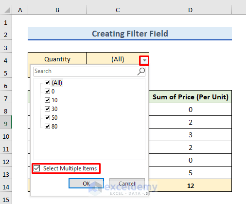
- Uncheck the zero.
- Click on OK.

- There are no zero values in the Quantity column of the pivot table.
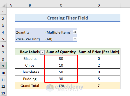
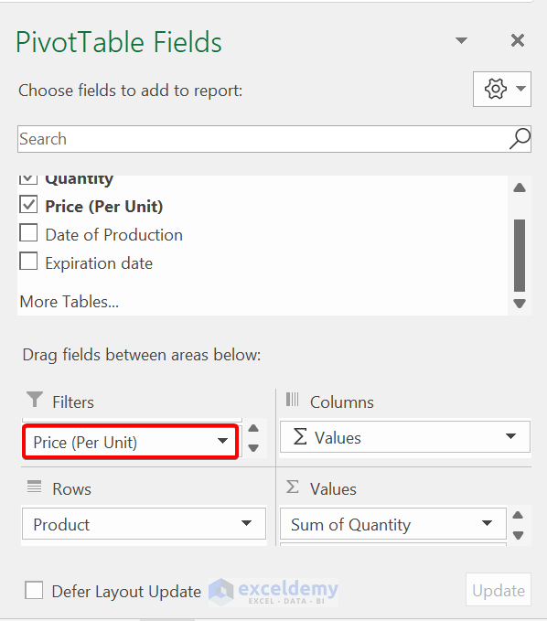
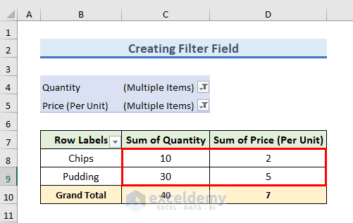
- Repeat the process for the Price(Per Unit) column.
- You can see that there are no zero values in the pivot table.
Method2 – Using the Filter Function on a Pivot Table
Steps:
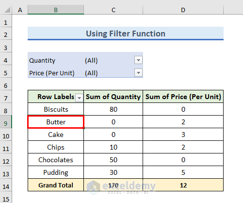
- Go to the Pivot Table.
- Select any element from the Row Labels. We have selected Butter.
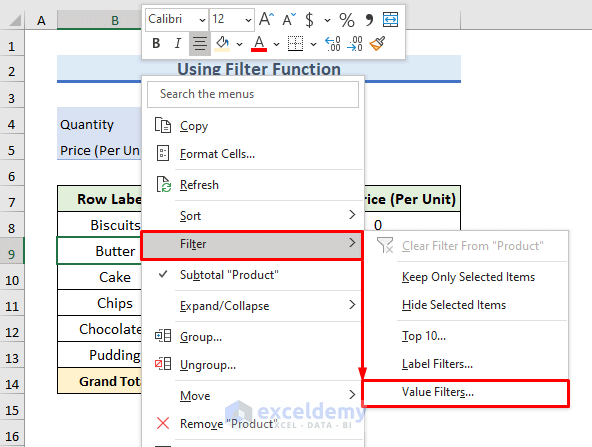
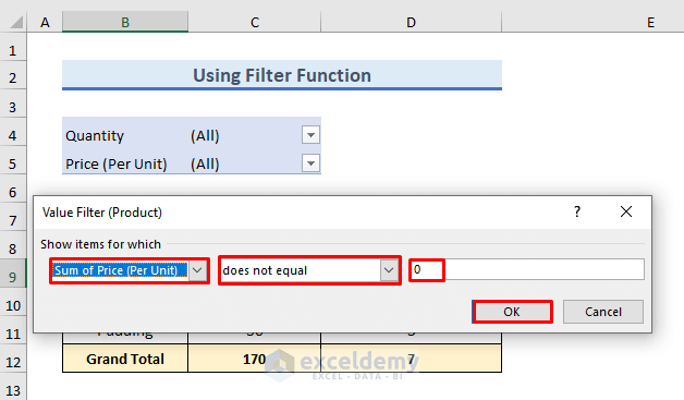
- Right-click on your mouse and select Filter, then choose Value Filter.
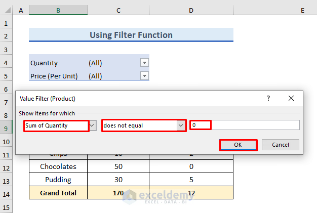
- Select a column. We are choosing the Sum of Quantity column.
- Select does not equal to from the dropdown menu.
- Type 0 (Zero) in the following empty field.
- Click on OK.
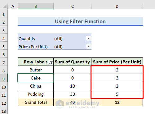
- There are no zero values in the Quantity column.
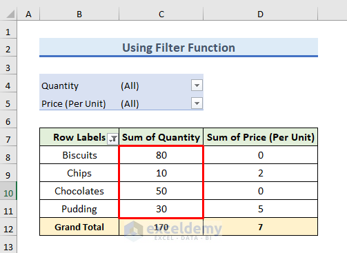
- Repeat the process for the Price column if you want.
- If you do, the table will look like the following figure.
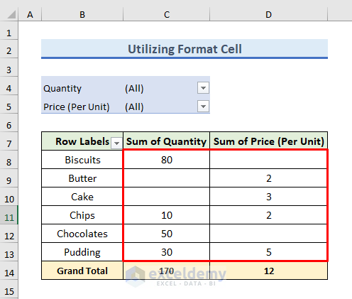
Method 3 – Hide Zero Values from a Pivot Table Using the Format Cells Command in Excel
Steps:
- Select the entire table.
- Press Ctrl + 1 on your keyboard to open the Format Cells dialog box.
- Go to the Custom panel.
- Clear General from the Type field.
- Paste the following code in the field and press OK:
0;-0;;@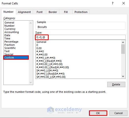
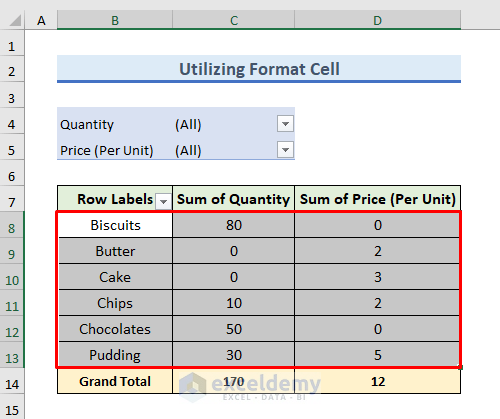
- There are no zero values in the pivot tables.
Things to Remember
- The second method will hide zero values from a particular column, not from the whole pivot table.
- The third method will hide zero values, not the cells or rows.
Practice Section
We have provided a Practice section on the right side of each sheet.
Download the Practice Workbook
Related Articles
<< Go Back to Blank in Pivot Table | Pivot Table Formatting | Pivot Table in Excel | Learn Excel
Get FREE Advanced Excel Exercises with Solutions!
