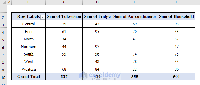
Consider this sample dataset in a pivot table with blank cells.
Method 1 – Use the Pivot Table Options to Remove Blank Rows
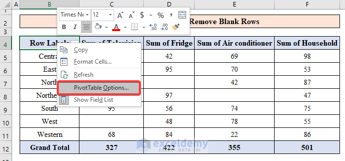
Step 1:
- Right-click the pivot table.
- Select “PivotTable Options”.
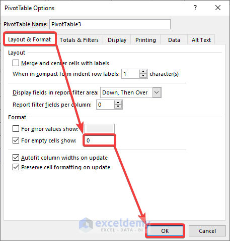
Step 2:
- Choose “Layout & Format”.
- In “For empty cells show”enter “0”.
- Click OK.
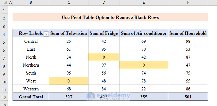
- All blank cells will display “0”.
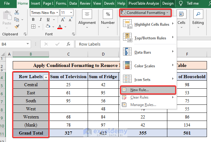
Method 2 – Applying Conditional Formatting to Remove Blank Rows in an Excel Pivot Table
Step 1:
- Select a range or group of cells.
- Go to Home and select “Conditional Formatting”. Choose “New Rule”.
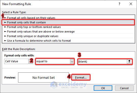
Step 2:
- In New Formatting Rule, click “Format only cells that contain”.
- In “Format only cells with:“, choose “equal to” and “(blank)”.
- Click “Format”.
Step 3:
- In the “Format Cells” dialog box will, choose “Number” and change the category to “Custom”.
- Enter “;;;”. This will format all zero or blank cells as blank.
- Click OK.
![]()
Step 4:
- Go to “Fill” and choose a color.
- Click OK.
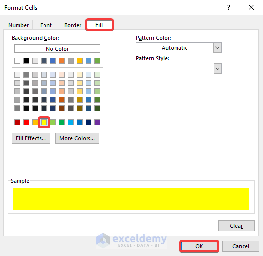
Blank is filled with color.
![]()
Method 3 – Utilizing the Filter Feature to Remove Blank Rows in an Excel Pivot Table
Steps :
- In a pivot table column header click the arrow.
![]()
- Uncheck blank.
- Click OK.
![]()
Blank rows will be removed.
![]()
Method 4 – Applying the Find & Replace Option to Remove Blank Rows in an Excel Pivot Table
Steps :
- Select the worksheet.
- Press Ctrl + H to see the “Find and Replace” dialog box.
- In “Replace with”, choose “Other”.
- Click “Replace All”.
![]()
- In the confirmation window,click OK.
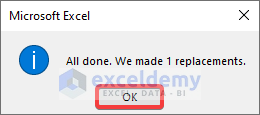
- Click “Close” to see the results.
![]()
Blank cells were removed.
![]()
Download Practice Workbook
Download this practice workbook to exercise.
Related Articles
<< Go Back to Blank in Pivot Table | Pivot Table Formatting | Pivot Table in Excel | Learn Excel
Get FREE Advanced Excel Exercises with Solutions!
