Step 1 – Create an Outline
- Create a sample template to enter data.
- Include Fixed Earnings and Variable Earnings.
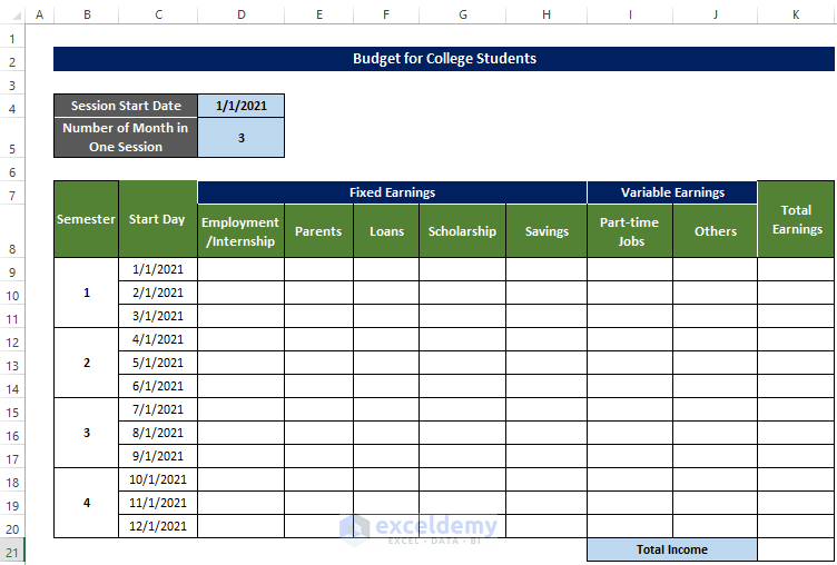
- Enter Variable fields and Fixed fields.
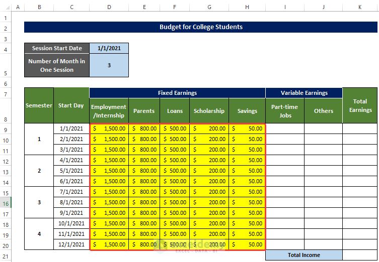
Step 2 – Enter the Fixed Earnings
- Enter fixed earnings:

- Include: Internships, allowances, loans (here 12 months), scholarships and savings.
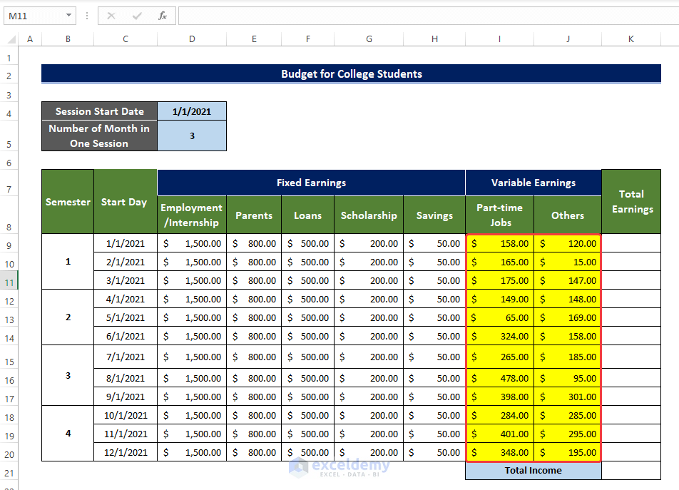
Step 3 – List Variable Earnings
- Include part-time jobs (consider different monthly income).
- Create an Others columns.
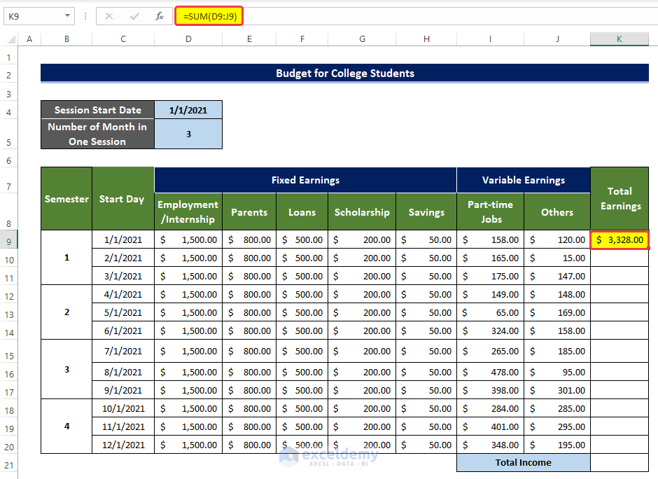
Step 4: Calculate the Total Income
- Select K9 and enter the following formula:
=SUM(D9:J9)
This is the output.
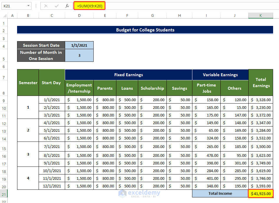
- Drag down the Fill Handle to see the result in the rest of the cells.
This is the output.

- Select K21 and enter the following formula:
=SUM(K9:K20)
This is the output.
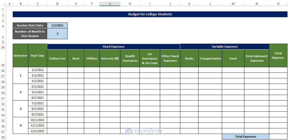
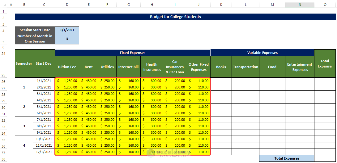
Step 5: Enter Fixed Expenses
- Include Tuition Fees, Rent Utility, Internet Bill, Health Insurance, Car Insurance, and Others in D26:J37.
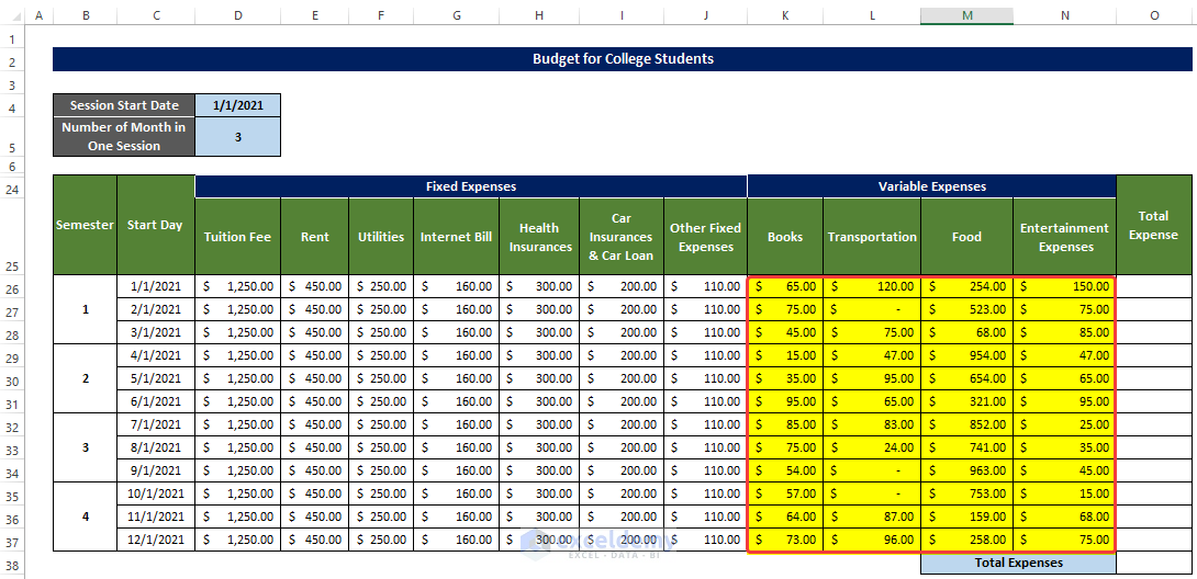
Step 6 – List Variable Expenses
- Include Books, Food, Entertainment and transportation (these expenses need to be updated every month).
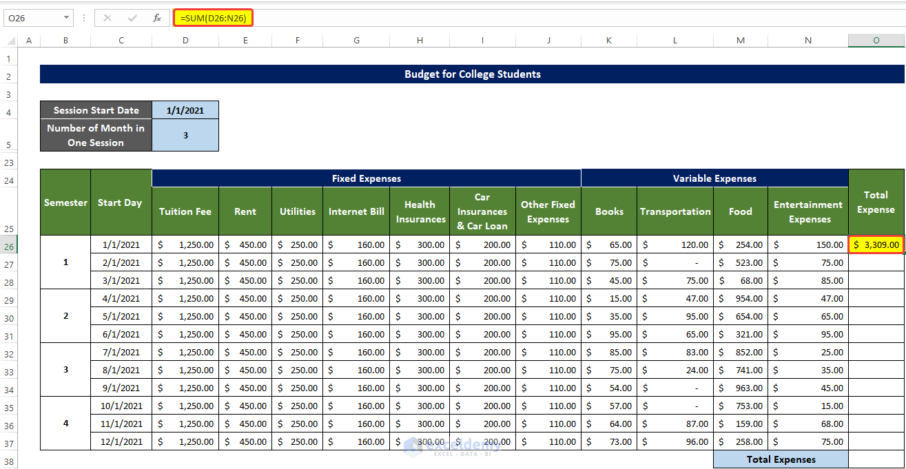
Step 7 – Calculate the Total Expenses
- Select O26 and enter the following formula:
=SUM(D26:N26)
This is the output.
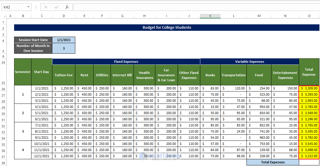
- Drag down the Fill Handle to see the result in the rest of the cells.
This is the output.
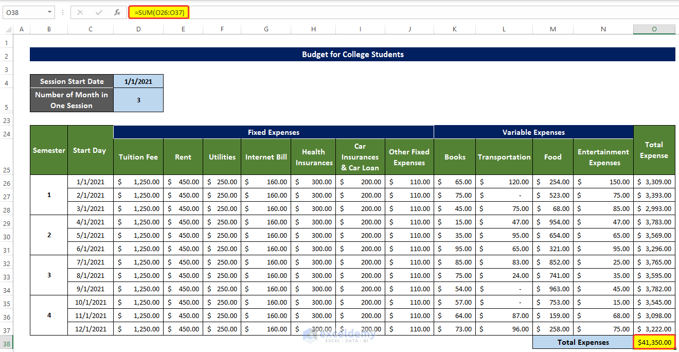
- Select O38 and enter the following formula:
=SUM(O26:O37)
- This is the output.
Step 8 – Calculate the Net Balance
- Selected I4 and enter the following formula:
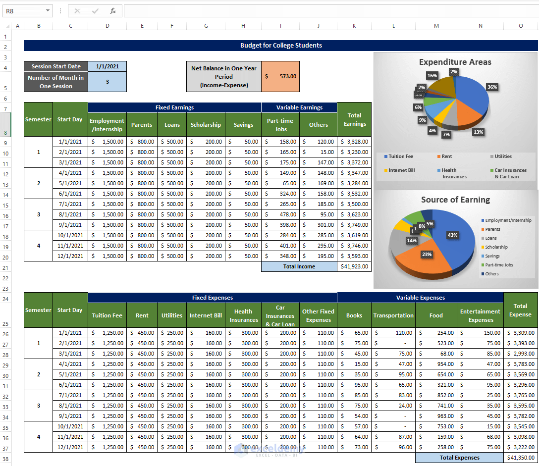
=K21-O38
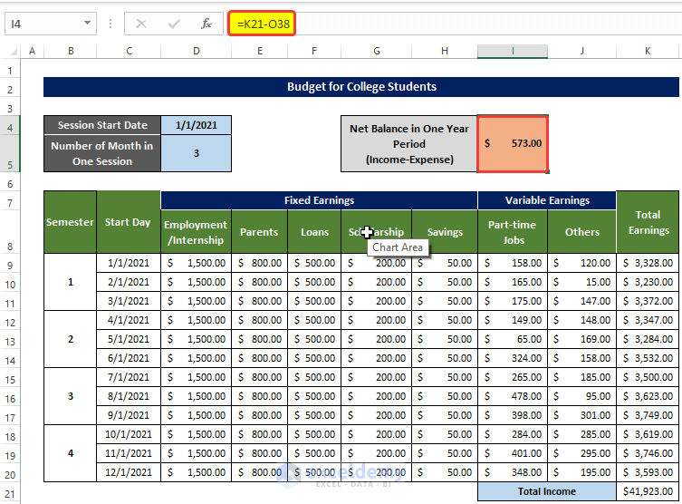
It Subtracts the Expenses from the Total Earnings.
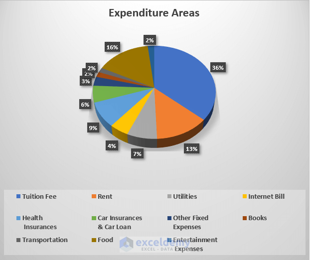
Step 9 – Generate the Final Budget with Charts
The PIe chart below showcases the income:

- The chart below showcases Expenses:
This is the final output:
Read More:How to Create a Personal Budget in Excel
Download the practice workbook.
Related Articles
- How to Make a Household Budget in Excel
- How to Make a Wedding Budget in Excel
- How to Make a Family Budget in Excel
<< Go Back To How to Create a Budget in Excel | Excel For Finance | Learn Excel
Get FREE Advanced Excel Exercises with Solutions!
