Method 1 – Prepare a Budget for a Company Manually
Step 1: Creating Basic Outlines to Prepare a Budget for a Company
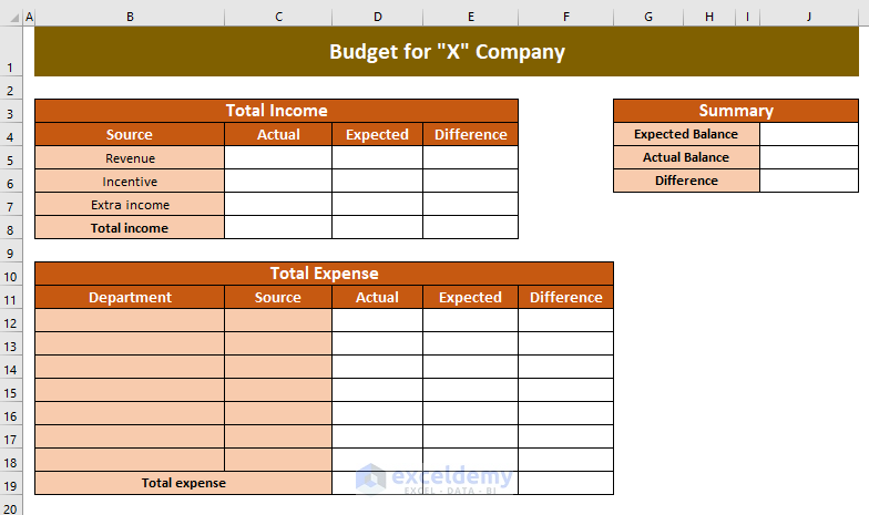
- Open a new workbook and create a worksheet: Budget.
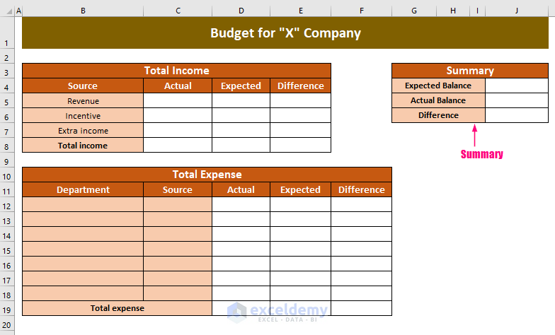
- Enter the header: Budget for “X” Company.
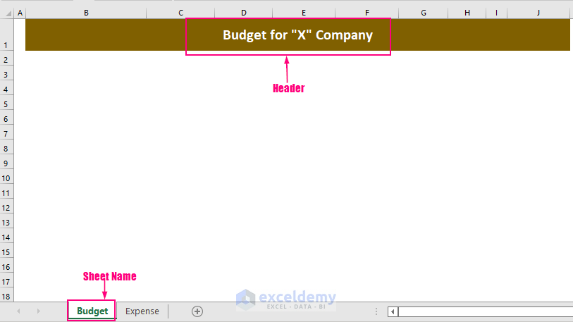
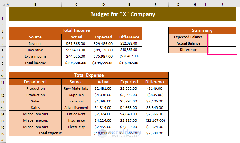
- Insert 3 tables for Income, Expense, and Summary.
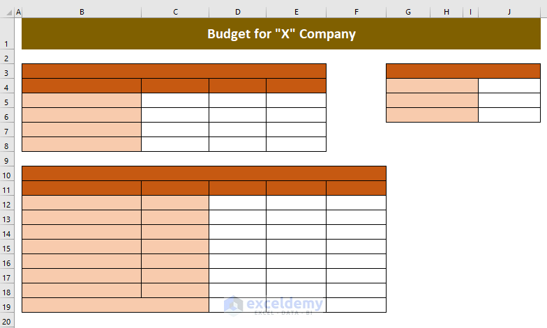
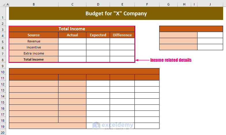
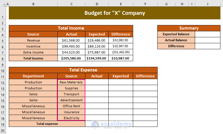
Enter the entities of income in the first table on the left side:
Here, Total Income as the header of the first table and 4 columns: Source, Actual, Expected, and Difference. Source of income includes: Revenue, Incentive, and Extra Income.
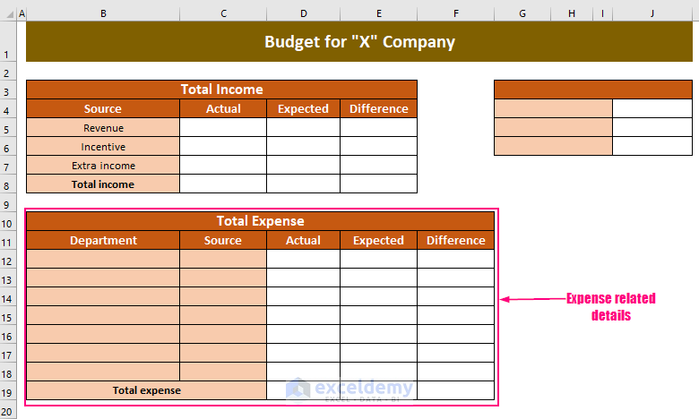
- The table below is the Total Expense table with 5 columns – Department, Source, Actual, Expected, and Difference.
The last table on the right side, is a Summary table with 3 rows: Expected Balance, Actual Balance, and Difference.
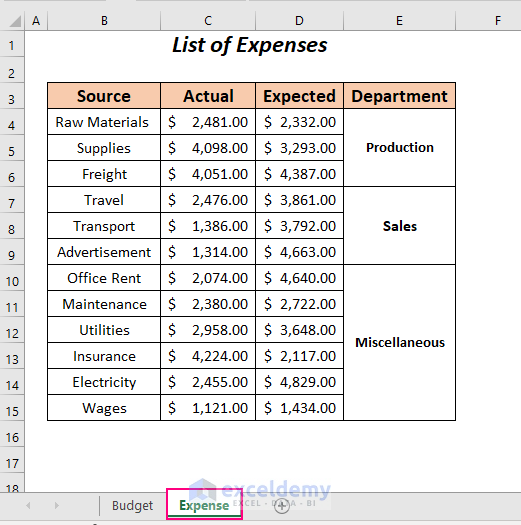
In the Expense sheet, all expenses of different departments are listed.
Read More: How to Prepare Annual Budget for a Company in Excel
Step 2: Calculate the Income
Calculate the total income and determine the differences between the actual income and the predicted income.
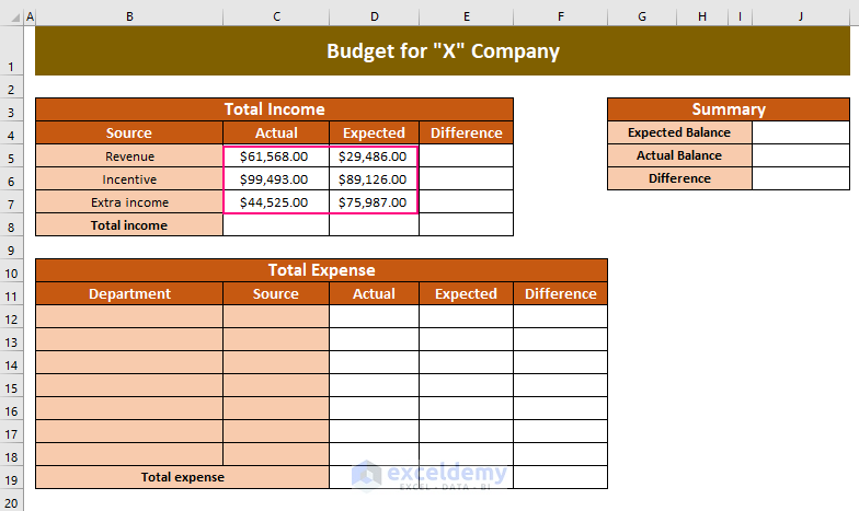
- Enter the actual and expected income from different sources in the Actual and Expected column.
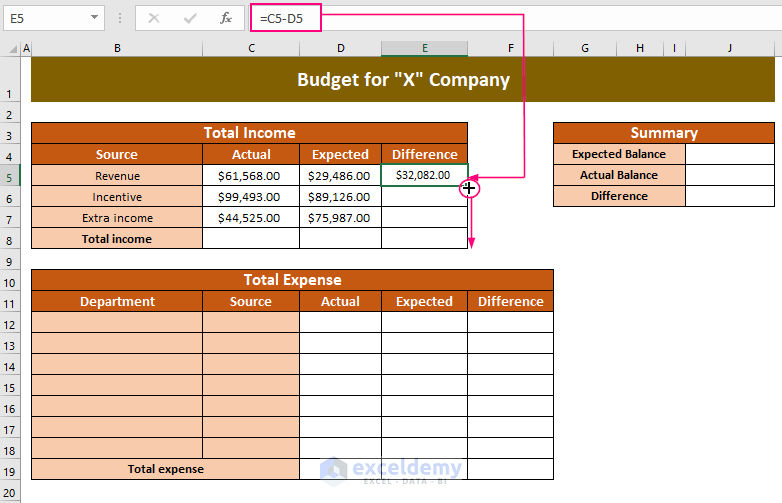
- Use the following formula in E5 and drag down the Fill Handle tool.
=C5-D5C5 is the Actual Income and D5 is the Expected Income (a subtraction is made)
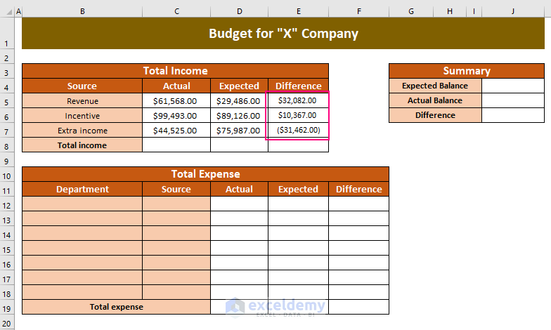
This is the output.
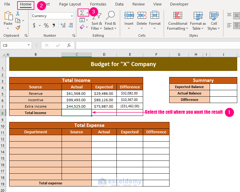
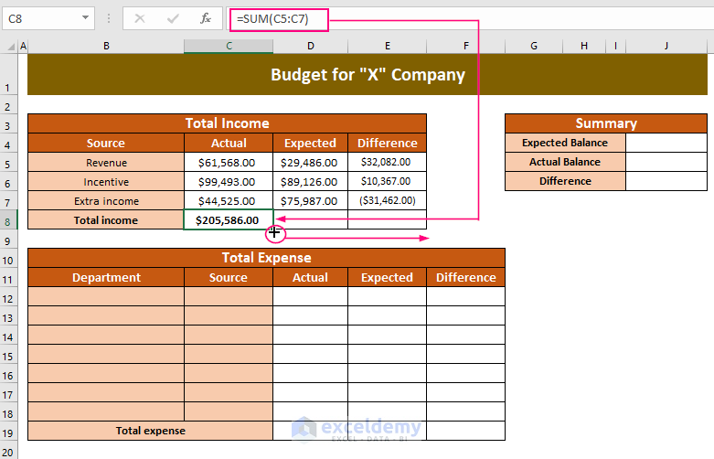
Use the AutoSum option to calculate the total income values automatically (if you add or delete any values, the total value will be updated).
- Select C8 to see the result.
- Go to the Home Tab >> Editing>> AutoSum.
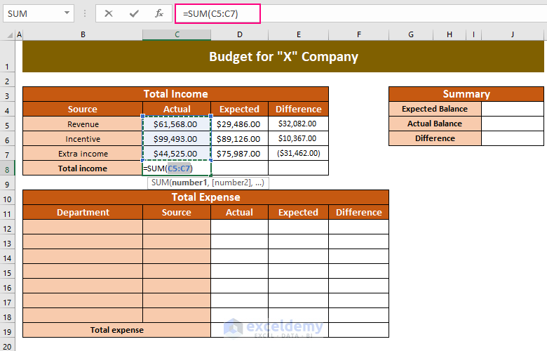
The following formula will be displayed in the cell.
=SUM(C5:C7)The SUM function calculates the sum in C5:C7.
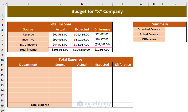
- Press ENTER and drag the Fill Handle to the right.
This is the output.
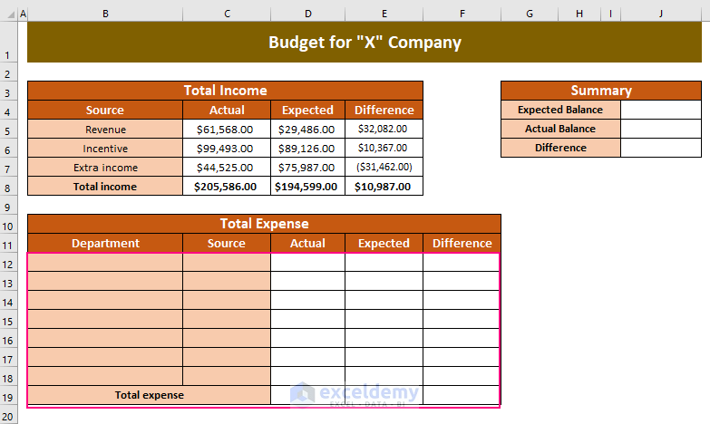
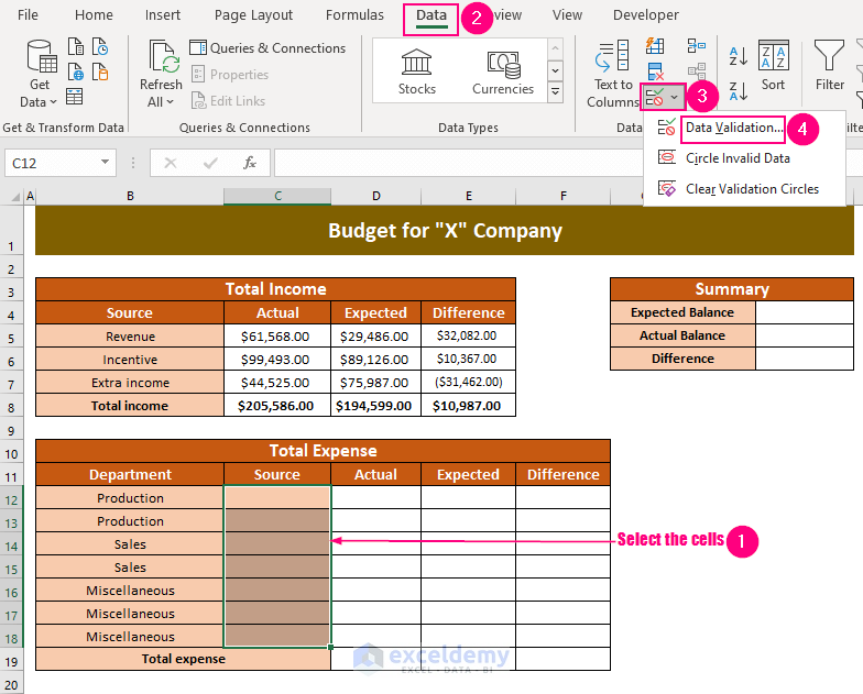
Step 3 – Creating a Dropdown List for Different Departments of Expenses
Calculate the total expenses and the differences between the actual and expected values.
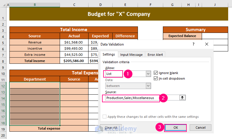
- Select all cells in the Department column and go to the Data Tab >> Data Tools >> Data Validation >> Data Validation.
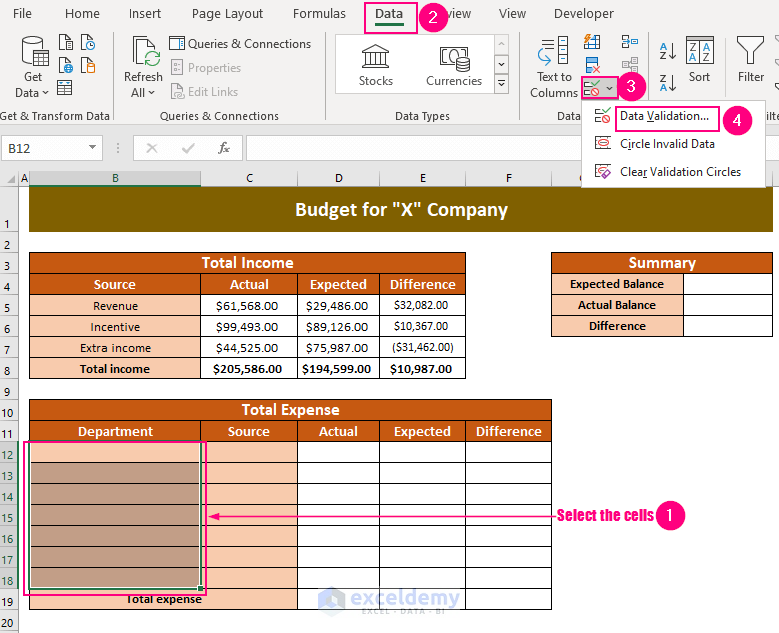
In the Data Validation wizard:
- Select List in Allow.
- In Source, enter the name of the departments separated by commas (here, Production, Sales, Miscellaneous).
- Click OK.
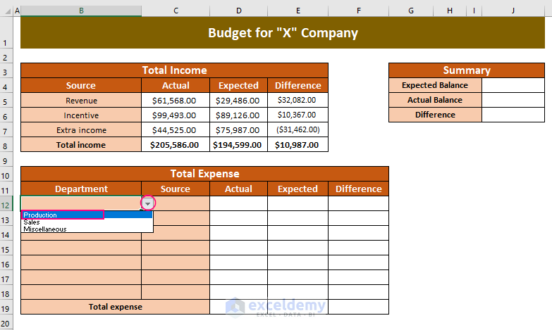
- Click the dropdown arrow in the Department column.
- Select a department from the list (here, Production for the first cell).
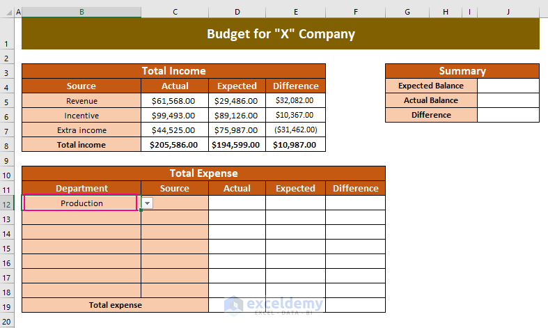
Production will be displayed in B12.
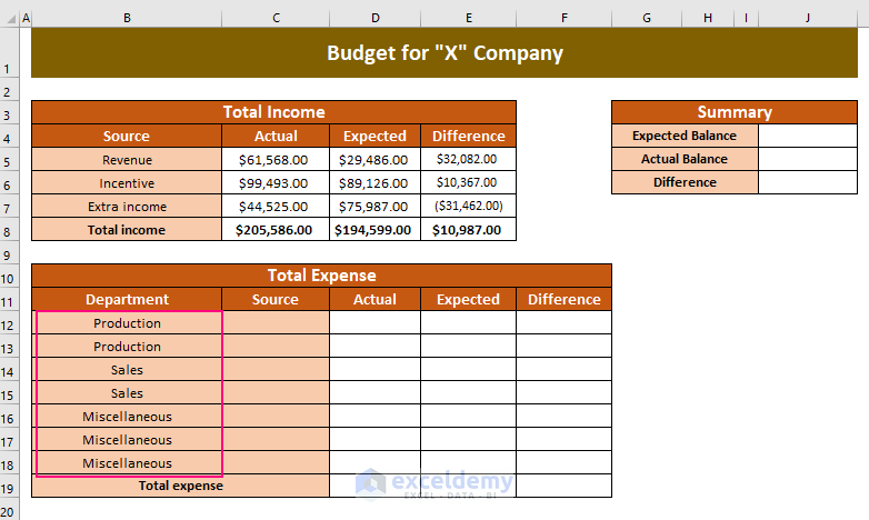
Repeat the procedure for other departments.
Read More: How to Create a Business Budget in Excel
Step 4: Creating a Dropdown List for Different Sources of Expenses
- To create a dropdown list for the Source column, select the column.
- Go to the Data Tab >> Data Tools >> Data Validation >> Data Validation.
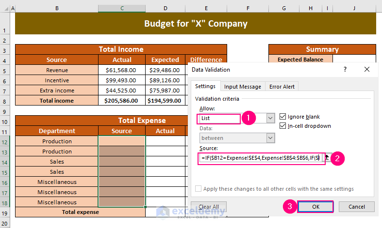
- In the Data Validation wizard, select List in Allow.
- In the Source box, enter the following formula.
=IF($B12=Expense!$E$4,Expense!$B$4:$B$6,IF($B12=Expense!$E$7,Expense!$B$7:$B$9,Expense!$B$10:$B$15))the IF function is used 2 times to create the Nested Loop effect.
- The first IF function checks if the value in $B12 matches the value in $E$4, in the Expense sheet. If there’s a match, it will return the values in $B$4:$B$6, in the Expense sheet. Otherwise, it will move to the next loop.
- The second IF function checks if the value in $B12 matches the value in $E$7, in the Expense sheet. If there’s a match, it will return the values in $B$7:$B$9, in the Expense sheet. Otherwise, the values in $B$10:$B$15 in the Expense sheet.
- Click OK.
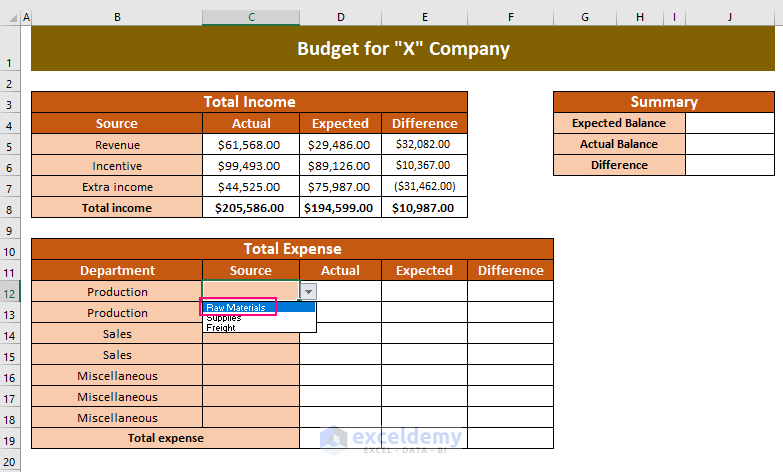
- Click the dropdown arrow in the Source column.
- Select a department from the list (here, Raw Materials for the first cell).
If you click the dropdown arrow in C16, whose corresponding cell in the Department column is Miscellaneous, you will see the source of expenses of this department in the list.
- Choose an option from the list (here, Office Rent).
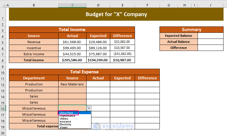
Office Rent will be displayed in C16.

Selected different sources to see the output.
Step 5: Calculate Expenses to Prepare a Budget
- Enter the following formula in D12 and drag down the Fill Handle tool.
=VLOOKUP($C12,Expense!$B$4:$D$15,2,FALSE)$C12 is the lookup value in the Source column, Expense!$B$4:$D$15 is the lookup range in the Expense sheet, 2 is the column number of this range, and FALSE is used for an exact match.
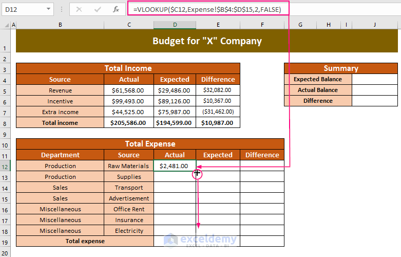
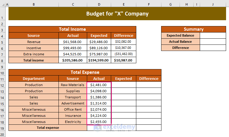
The actual expenses are displayed in the Actual column.
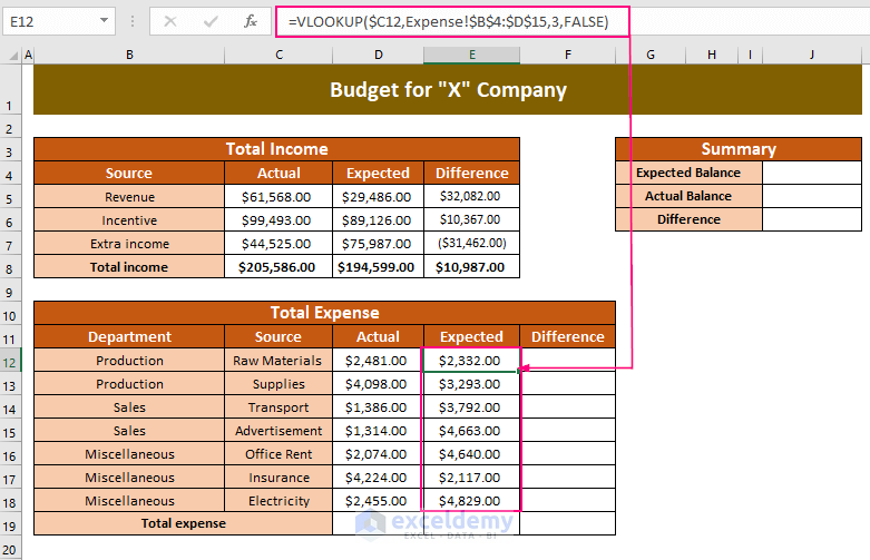
Use the following formula to get the Expected Expenses from the Expense sheet.
=VLOOKUP($C12,Expense!$B$4:$D$15,3,FALSE)$C12 is the lookup value in the Source column, Expense!$B$4:$D$15 is the lookup range in the Expense sheet, 3 is the column number of this range, and FALSE is used for an exact match.
- Use the following formula in F12 and drag down the Fill Handle tool.
=E12-D12E12 is the Expected Expense and D12 is the Actual Expense (to calculate the difference, subtract the expected value from the actual value).
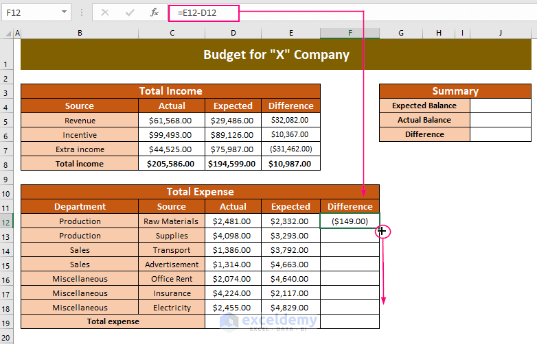
The differences are displayed in the Difference column.

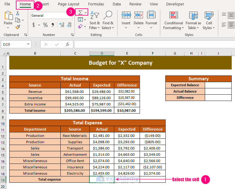
- Select D19 to see the total result and go to the Home Tab >> Editing>> AutoSum.
- Press ENTER and drag the Fill Handle tool to the right.
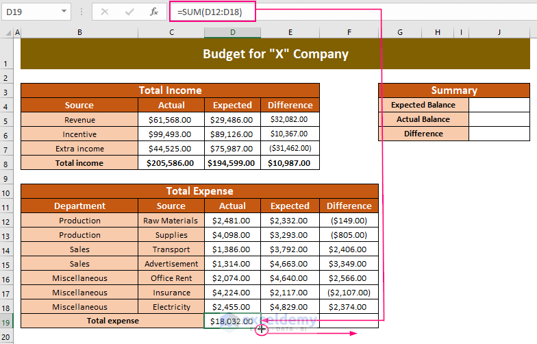
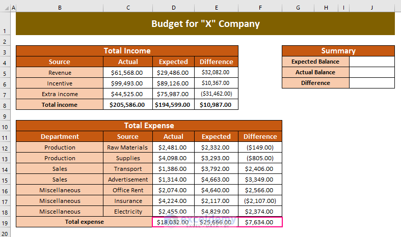
Total expenses are calculated.
Step 6: Budget Summary Calculation
Calculate the remnant balance.
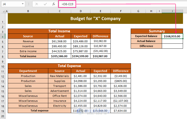
- Enter the following formula in J4.
=D8-E19D8 is the Expected Income and E19 is the Expected Expense, their difference will return the Expected Balance.
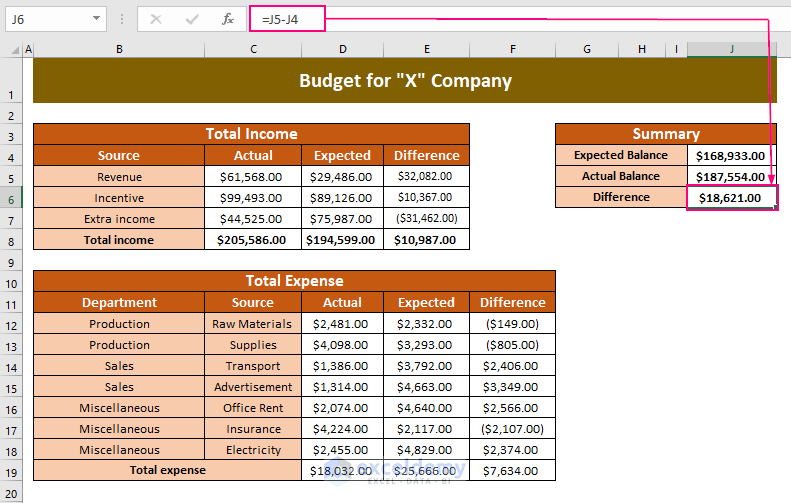
- Use the following formula in J5.
=C8-D19C8 is the Actual Income and D19 is the Actual Expense, their difference will return the Actual Balance.

- To see the differences between these balances, use the following formula in J6.
=J5-J4J5 is the Actual Balance and J4 is the Expected Balance, their difference will return the Difference.
Step 7: Plotting Income and Expense Values
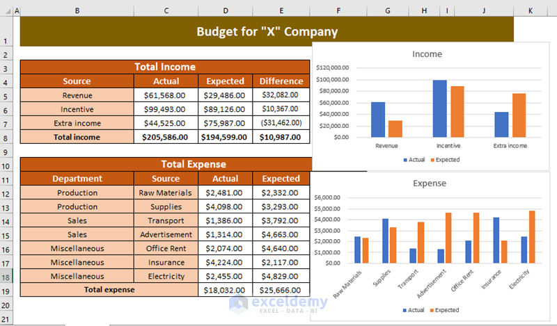
 For the income, select the actual and expected income values with their sources and go to the Insert Tab >> Charts>> Insert Column or Bar Chart >> select a column chart (here, 2-D Column).

- Name the chart: Income.
This is the output.

Select the values of the expenses and create an Expense chart:
Method 2 – Prepare a Budget for a Company Using an Excel Template
- Open a new workbook and go to the File tab.
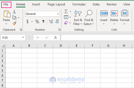
- Select New.
- In the right pane, select Budgets.
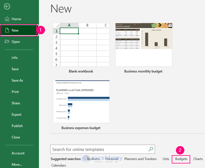
- Select an option. Here, Monthly Company Budget.

- Select Create.

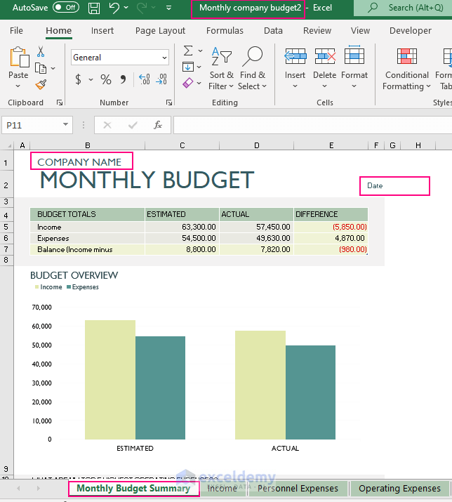
- A new workbook will be created with 4 sheets – Monthly Budget Summary, Income, Personnel Expenses, Operating Expenses.
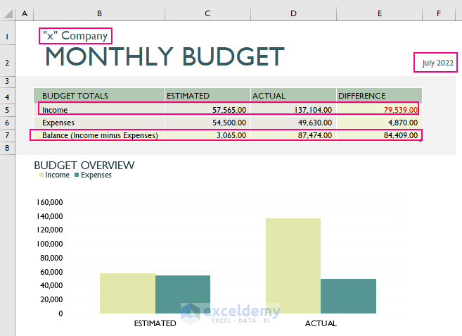
- The first sheet contains the summary budget with its graphical representation. Enter the company name and date.
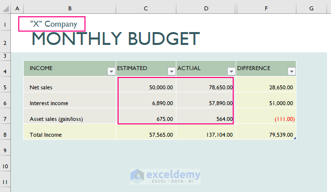
- In the Income sheet, change numbers and sources.

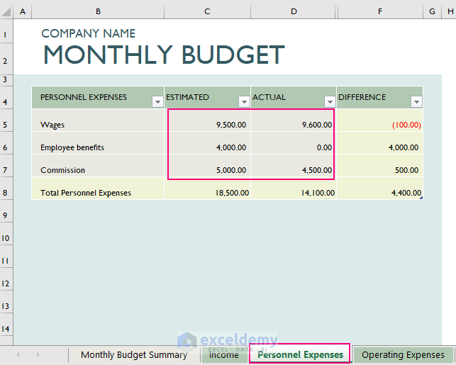
- Change expenses in the Personnel Expenses sheet.
- In the Operating Expenses sheet, change sources and values.
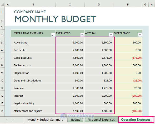
This is the output.
Because the values in the Income sheet were changed, the Monthly Budget Summary sheet and the total balance also changed.
The company name was added, as well as the current date (05/07/2022).
Read More: How to Create an Operating Budget in Excel
Download Workbook
Related Articles
<< Go Back To How to Create a Budget in Excel | Excel For Finance | Learn Excel
Get FREE Advanced Excel Exercises with Solutions!
