Insert Drop Down Calendar in Excel Without Date Picker

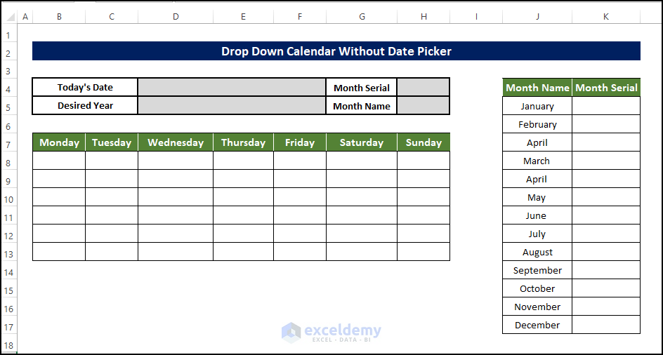
Step 1 – Prepare Calendar Layout

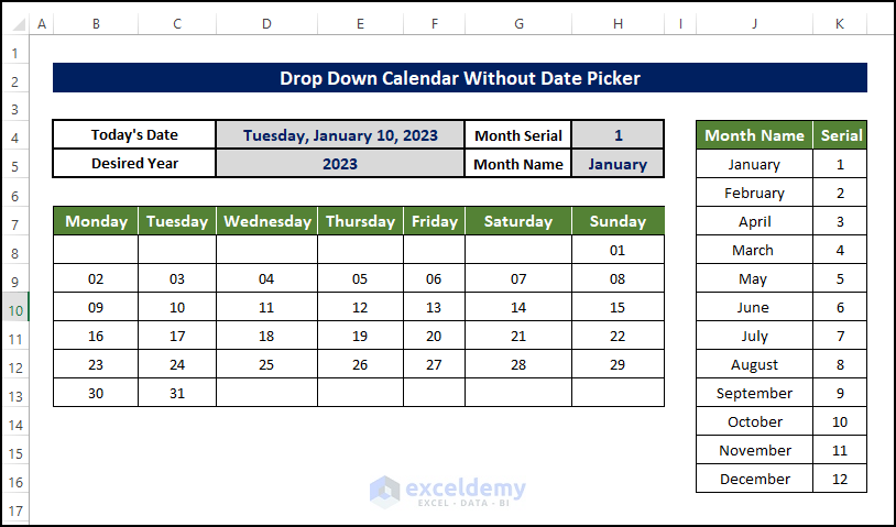
• Prepare the layout of the outline of the calendar.
• Place the date and month on the sheet.
• The date and the month should be dynamic to current date.
• The calendar will follow the weekdays starting from the Monday
• All the month’s names are in the range of cell J4:J17.

Read More: How to Use Excel UserForm as Date Picker

Step 2 – Insert Drop Down List of Months

• To add a drop-down list, select cell H5.
• Go to Data > Data Tools > Data Validation > Data Validation.

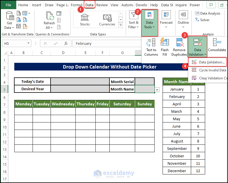
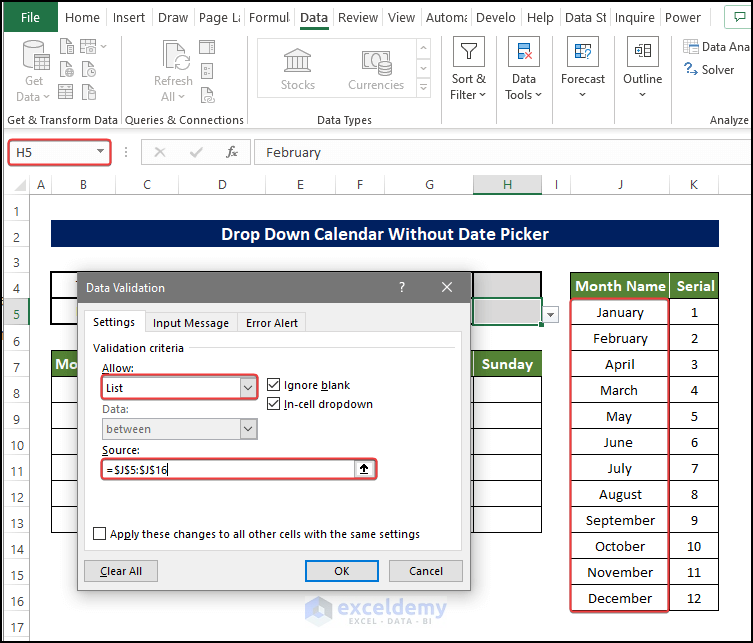
• In the Data Validation window, go to the Settings
• Select List in the drop down to allow
• Select the range of cells J5:J16 in the source range box.
• Press OK.

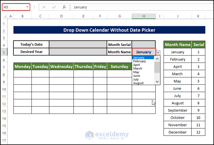
• We can see the month names in cell H5 in the form of a drop-down list.

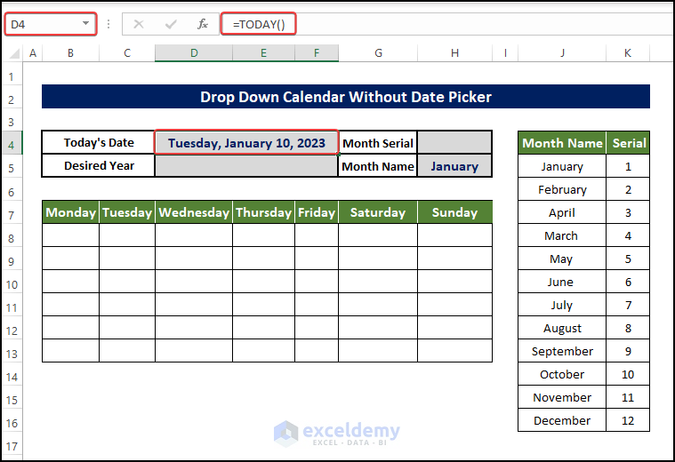
Step 3: Formulize Calendar Outline

• To extract the current date in the dataset, select cell D4, and enter the following formula:

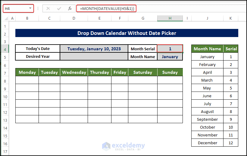
• Select cell H4 and enter the following formula:

• Press Enter to see the month’s serial in cell H4.

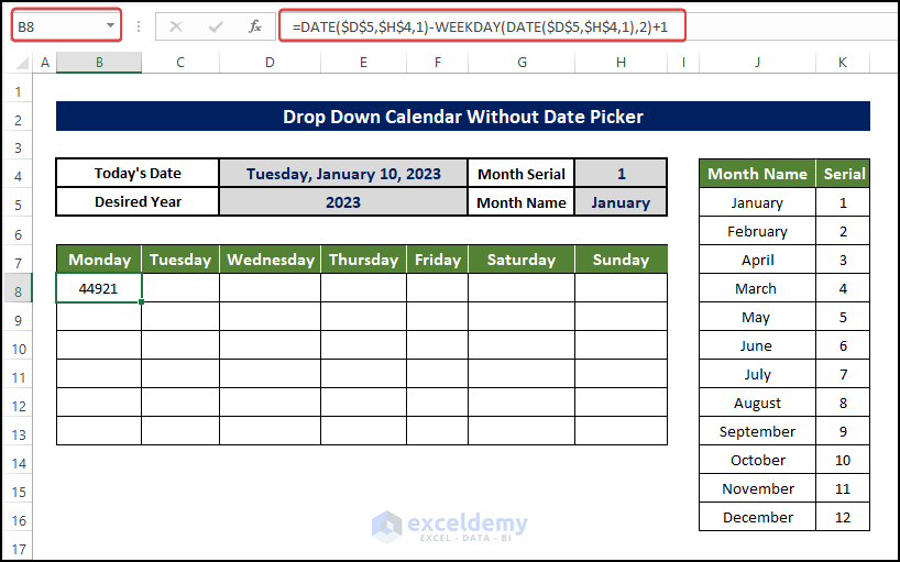
• Enter 2023 in cell D5.
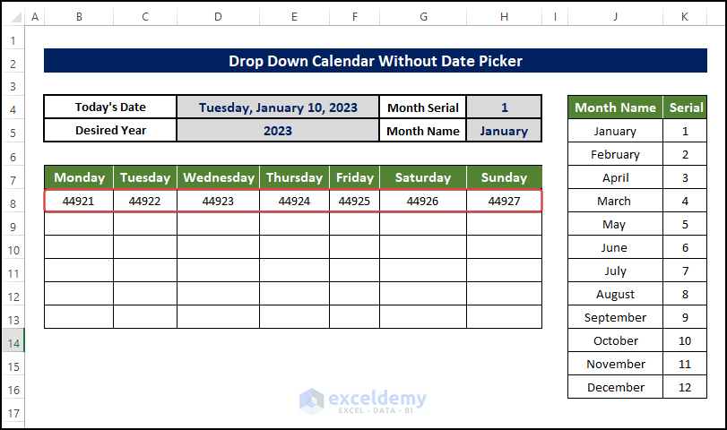
• Select cell B8 and enter the following formula:

• Press Enter to see that first date appear in cell B8.

• Select cell C8 and enter the following formula:

• Press Enter to see the result in cell C8.

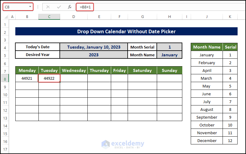
• Drag the fill handle from cell B8 to cell H8
• This will fill the range of cells with dates starting from the 29th of October to the 4th of September.

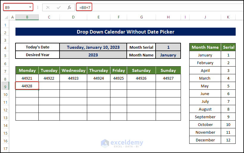
• Select cell B9 and enter the following formula:

• Press Enter to see the result in cell B9.

• Drag the Fill Handle to cell B13.

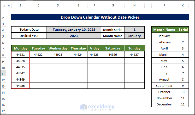
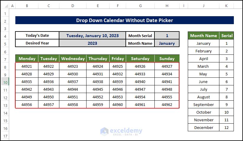
• Repeat the same process for the rest of the cells.
• The result shows the dates for all of the weekdays in a month.

Read More: Make an Alternative to Datepicker in Excel

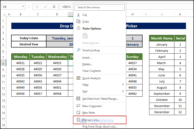
Step 4: Reformat Data Values

• Right-click and choose Format Cells.

• In the Format Cells window, go to the Number
• In the Custom options, select the Type
• In the Type field, enter “dd”
• This will allow the user to see only the day portion of the date.
• Click OK.

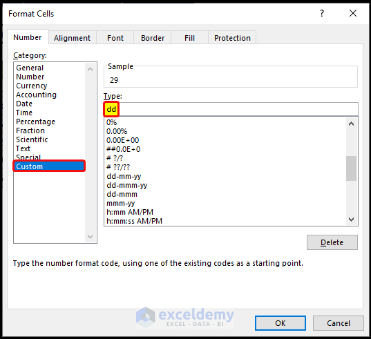
• The calendar will now have the dates in a double-digit format.
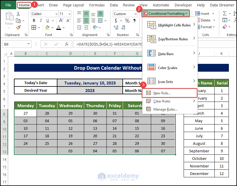
• We have the dates from the previous and next month.
• To avoid that, we need to conditionally format the values.
• Select the whole calendar and go to the Home tab > Conditional Formatting > New Rule.

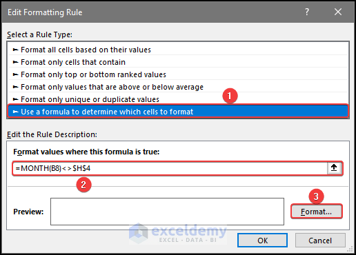
• In the Edit Formatting Rule window, select Use a Formula to Determine Which Cells to Format.
• Enter the following formula:

• Click on the Format button.

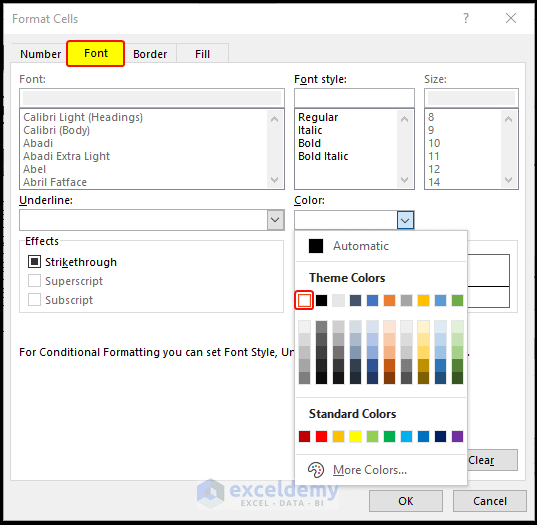
• In the Format Cells dialog box, click on the Fill
• In the Fill tab, choose the color white as the fill color.
• Switch to the Font tab and choose the Color white as the font color.
• Click OK.

• The dates from the other months are now omitted from the view.
• Enter the desired year and month from the drop-down list to get the calendar to display the exact same weekdays of months and year.

Read More: [Solved!] Datepicker Not Showing in Excel

Download Practice Workbook

Related Articles

• How to Use Date Picker in Excel 64-Bit
• Excel Date Picker for Entire Column
• How to Insert Calendar in Excel Cell

<< Go Back to Excel Date Picker | Learn Excel