How to Use the SUM Function in Google Sheets (8 Easy Examples)

Image by Editor | Midjourney
 

The SUM function is the fundamental function in Google Sheets. It is one of the most used and powerful functions. It allows you to quickly add up a large range of cells whether it’s your daily expense data or any sales data. It saves time and manual errors. In this article, we will show how to use the SUM function in Google Sheets.

Understanding the SUM Function

The SUM function adds all numbers in a selected range of cells and automatically updates the sum if any changes occur in any of the values of ranges.

Syntax:

=SUM(value1, [value2, ...])

• value1: The first number or range to be added.
• value2, … (optional): Additional numbers or ranges you want to add.

Notes:

• If only a single number for value1 is supplied, SUM returns value1.
• Although SUM is specified as taking a maximum of 30 arguments, Google Sheets supports an arbitrary number of arguments for this function.

1. Summing up a Range of Cells

Using the SUM function, you can calculate the total sales for Products from Quarter 1 to Quarter 4.

• Select cell F2 and insert the following SUM function.
• Press Enter.
• Drag the formula down to apply it to the rest of the cells.

Formula:

=SUM(B2:E2)

This formula adds up the Quarterly sales of Product A.

2. Combining Ranges and Individual Values

You can mix individual values with cell ranges. Let’s use a dataset you can use for the example of quarterly sales where you combine ranges and individual values.

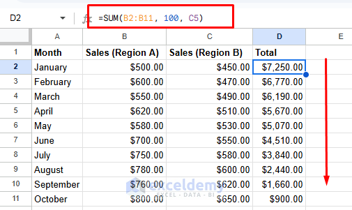
• Select cell D2 and insert the following SUM function.
• Press Enter.
• Drag the formula down if you want to apply it to additional rows.

Formula:

=SUM(B2:B11, 100, C5)

This formula sums up the quarterly sales from Region A (January to October). Adds a constant value of 100. Then, add the sales value from Region B for May.

3. Summing an Entire Column

To get the total sales of all products for January:

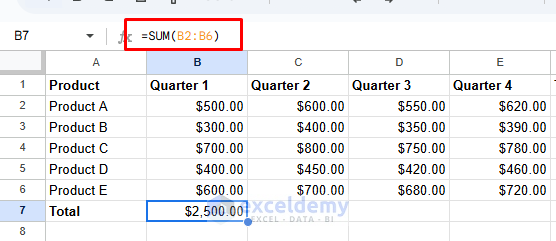
• Select cell B7 and insert the following formula.
• Press Enter.

Formula:

=SUM(B2:B6)

This formula sums up the Quarterly 1 sale.

4. Summing Multiple Ranges

To calculate the total sales for quarters 1 and 2 combinedly, you can use the SUM function.

• Select cell H2 and insert the following formula.
• Press Enter.

Formula:

=SUM(B2:B6, C2:C6)

This formula adds all values from two different column ranges. Which will be Quarterly 1 and 2 sales for the product.

5. Using Auto-Sum Feature

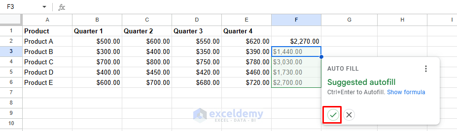
You can use the AutoSum feature in Google Sheets to bring the sum function automatically.

• Select cells B2 to B6.
• Click Insert >> select the Functions button on the toolbar.
• Select SUM from the dropdown list.

• The total appears automatically in the next cell F2.

• Google Sheets offers autofill suggestions. Click on the Tick mark to autofill the result in the rest of the cells.

6. Conditional SUM Using SUMIF

To sum up sales of products that sold more than 600 units in all quarters, you can use the conditional sum.

• Select cell F2 and insert the following formula.
• Press Enter.

=SUMIF(B2:E2, ">500")

This formula sums up the values where quarterly sales are greater than 500.

7. Using SUM with Individual Numbers

You can also sum specific numbers directly in Google Sheets.

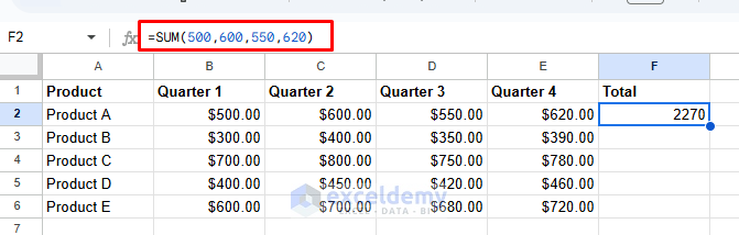
• Select cell F2 and insert the following formula.
• Press Enter.
• Drag the formula down if you want to apply it to additional rows.

Formula:

=SUM(500,600,550,620)

This formula sums up the quarterly sales for Product A.

8. Summing Visible Cells Only Using SUBTOTAL

If some cells are hidden, SUM will still count them. To sum up only visible cells:

• Select cell B7 and insert the following formula.
• Press Enter.

Formula:

=SUBTOTAL(9,B2:B6)

In this formula, 9 stands for the SUM function within SUBTOTAL.

Common Errors

• #VALUE! Error: If the range of cells contains text that cannot be converted to numbers.
• Wrong Range: Double-check the selected range to ensure it’s correct.
• Text values in your range: The SUM function ignores text. If cell A1 contains “100” as text (often left-aligned rather than right-aligned), it won’t be included in the sum.
• Formatting issues: Numbers stored as text won’t be calculated. You might need to convert them using the VALUE function.
• Hidden zeros: Sometimes cells appear empty but contain zero values. SUM will count these zeros.

Conclusion

Google Sheets’ SUM function is essential to quickly add numbers from different ranges, based on conditions, etc. With the examples provided, you can now apply this function to a variety of real-world scenarios. By mastering the SUM function, you’ve taken your first step toward proficiency in Google Sheets. Remember that this function forms the foundation for more advanced functions like SUMIF and SUMIFS.