How to Make Excel Go to the Next Line Automatically (2 Methods)

Method 1 – Enabling the Wrap Text Feature

• Click on the cell containing the sentence you want to split into multiple lines (e.g., Cell B5).

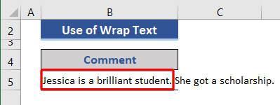
• Ensure that the width of the cell is insufficient to accommodate the entire sentence.
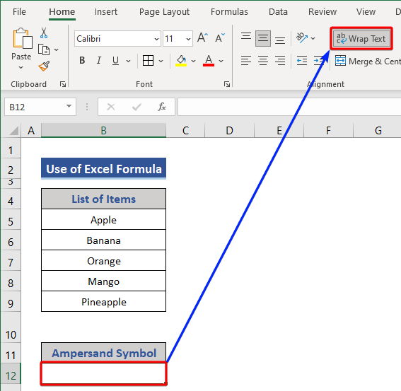
• Click the Wrap Text feature from the Alignment group.

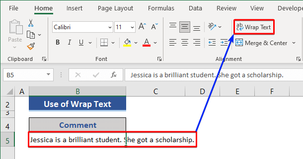
• The sentence will now appear on multiple lines within the cell.

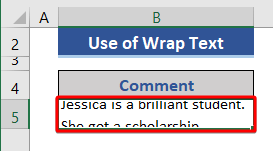
• Adjust the cell’s length and width by dragging the column and row or using the AutoFit feature.

Read More: How to Space Down in Excel

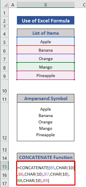
Method 2 – Using Excel Formulas to Join Text and Automatically Go to a New Line

The CONCATENATE function joins several text strings into one text string.

The TEXTJOIN function concatenates a list or range of text strings using a delimiter.

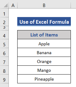
• In your dataset (e.g., a list of fruits), create a new row for applying a formula.

• Enable Wrap Text for the cell where you’ll apply the formula (e.g., Cell B12).

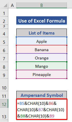
• Insert the following formula in Cell B12 using the ampersand symbol:

This formula joins the text strings (fruits) and adds new lines (CHAR(10)) between them.

• Press Enter to see the new lines added to the cell.

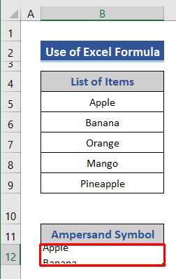
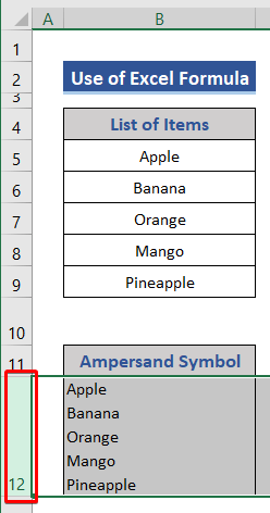
• Adjust the length of Cell B12 as needed.

Alternatively, you can use other functions like CONCATENATE or TEXTJOIN for similar results.

• Insert the below formula, based on the CONCATENATE function, in Cell B15 with Wrap Text

• Insert the below formula, based on the TEXTJOIN function, in Cell B15 with Wrap Text

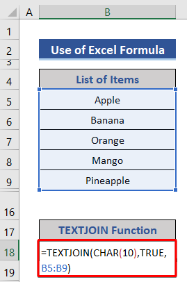
After applying any of these formulas we need to adjust the length of the corresponding cell and enable Wrap Text.

Read More: How to Do a Line Break in Excel

How to Insert a Line Break

Steps:

• Open the Excel file containing the dataset.  Our dataset is one sentence in a single cell.

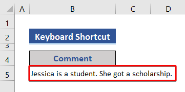
• Locate the cell with the sentence you want to split into multiple lines.
• Press F2 to make the cell editable.
• Move the cursor to the position within the sentence where you want to add a line break.

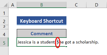
• Press Alt + Enter on your keyboard.

• A new line will be added within the cell.

• You’ll notice that the Wrap Text feature is enabled for this cell.
• Adjust the cell width as needed to display the multiline content properly.

How to Add a New Line in the Formula Bar

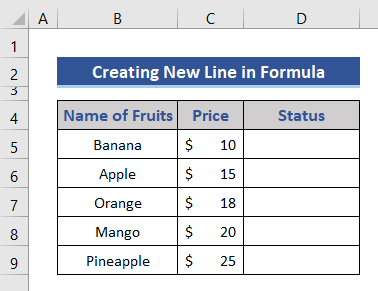
We’ll use the following dataset:

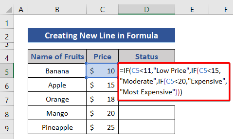
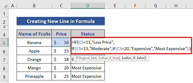
• Enter the following formula in a cell (e.g., Cell D5).

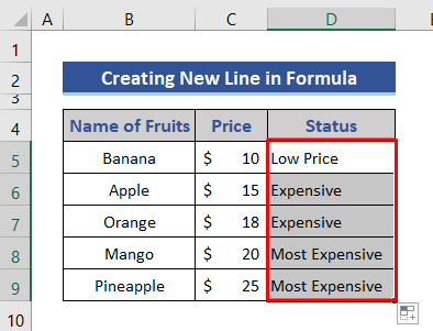
• Press Enter and then drag the Fill Handle icon.

• Edit the formula in Cell D5 by pressing the F2 button (for longer formulas, we press F2 to edit the formula).
• Place the cursor where you want to add a new line.
• Press Alt + Enter to insert a line break.

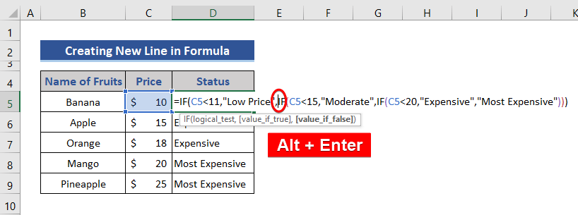
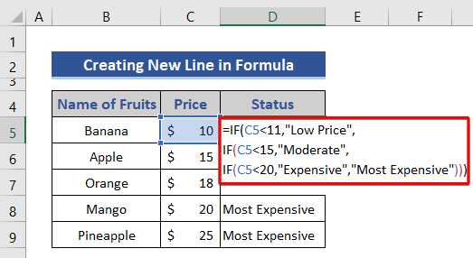
• We can see a new line is added to the formula.

• Repeat this process to add additional lines within the formula.

How to Create New Lines After a Specific Character in an Excel Cell

Using Find & Replace:

• Select the cells (Range B5:B6) where you want to insert line breaks.

• Press Ctrl + H to open the Find and Replace dialog.

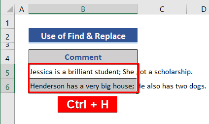
• In the Find what field, enter the semicolon symbol (;).
• In the Replace with field, press Ctrl + J.
• Click Replace All.

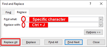
• We will see the number of replacements in the pop-up.

• The cell content will now have new lines after semicolons.

Read More: Find and Replace Line Breaks in Excel

Things to Remember

• Remember to ensure that the Wrap text feature is enabled to display the multiple lines correctly.
• If needed, adjust cell width manually.

Download Practice Workbook

You can download the practice workbook from here:

Related Articles

• How to Replace a Character with a Line Break in Excel
• How to Remove Line Breaks in Excel
• [Fixed!] Line Break in Cell Not Working in Excel
• How to Replace Line Break with Comma in Excel

<< Go Back to Line Break in Excel | Text Formatting | Learn Excel