How to Build a Full Calendar Interface in Excel Using Form Controls

 

Excel offers built-in features and formulas where you can build a full calendar without using any code. You can use form controls to create a dynamic calendar interface in Excel that users can navigate through different months and years.

In this tutorial, we will show how to build a full calendar interface in Excel using form controls.

Enable the Developer Tab

If the developer tab is not available in the ribbon panel, you will need to enable it from the Customize Ribbon option.

• Go to the File tab >> select Options.
• Select Customize Ribbon.
• Check the Developer box in the right panel.
• Click OK.

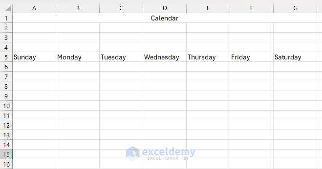
Step 1: Create the Worksheet Layout

Create the Worksheet Layout:

• Open a new Excel workbook.
• Create a new worksheet and rename it to “Calendar”.
• Set up the basic structure:
  • Row 1: Title area of calendar.
  • Row 3: Month and Year controls.
  • Row 5: Day headers (Sun, Mon, Tue, etc.).
  • Rows 6-11: Calendar grid (6 rows to accommodate all possible month layouts).

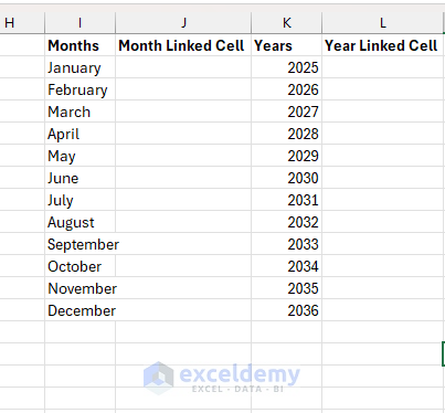
Create Day Headers and List Month and Years:

• Enter a list of months (e.g., Jan through Dec).
• List your desired years (e.g., 2025, 2026 to 2036).
• List day headers (e.g., Sun, Mon, through Sat).

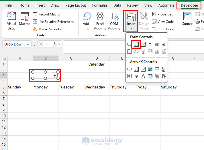
Step 2: Create the Date Controls

• Go to Developer tab >> select Insert >> select Form Controls.
• Select Combo Box (not ActiveX version).
• Draw the combo box in cell B3.

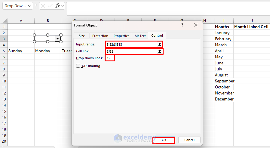
• Right-click the combo box >> select Format Control.

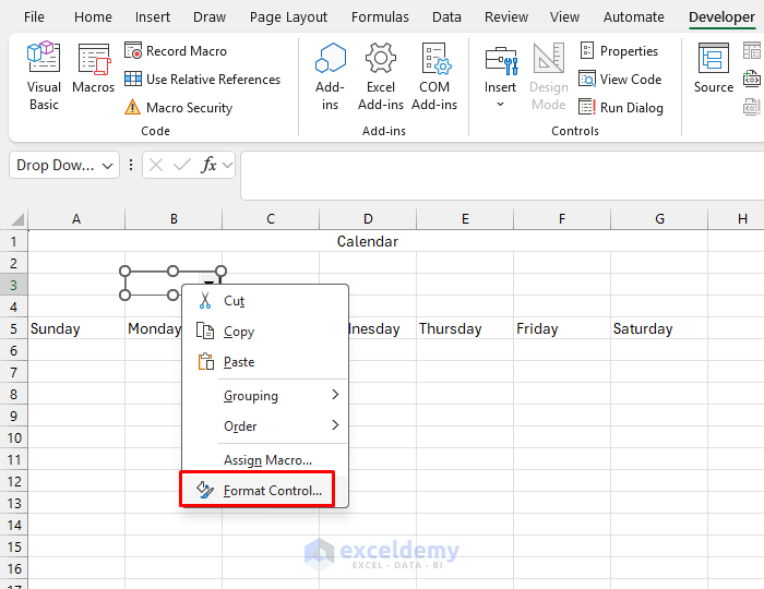
• In the Format Object box:
  • Input range: Select a list of months from column I (I2:I13).
  • Cell link: J2 (this will store the selected month number).
  • Dropdown lines: 12.
  • Click OK.

Add Year Selection Dropdown:

• Insert another Combo Box in cell D3.
• In the Format Object box:
  • Input range: Select the year list from column K (K2:K12 with years 2020-2039).
  • Cell link: L2 (this will store the selected year number based on the starting year).
  • Dropdown lines: 10.
  • Click OK.

Step 3: Set Up Helper Cells to Create Calendar Logic

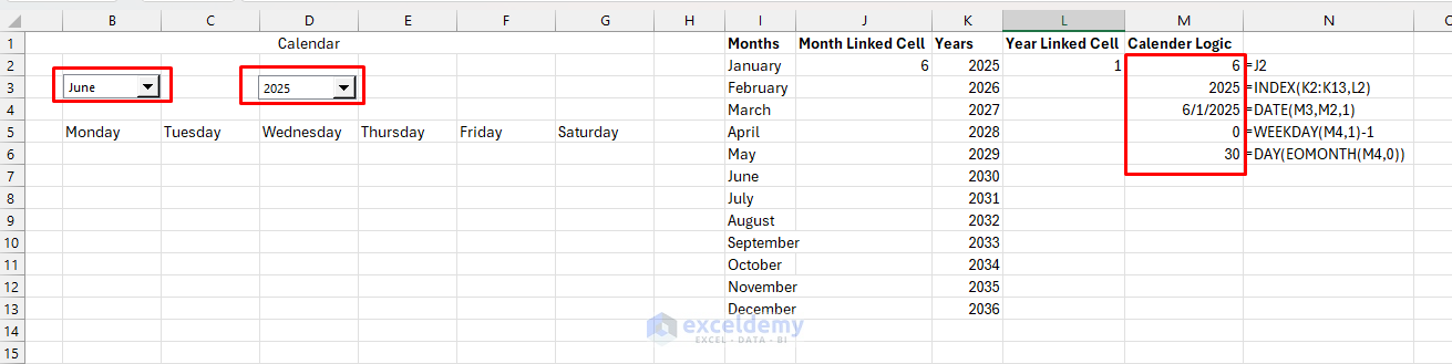
Create the helper formulas in column M.

Current Month Number:

• Select cell M2 and insert the following formula.

=J2

Current Year:

• Select cell M3 and insert the following formula.

=INDEX(K2:K13,L2)

First Day of Month:

• Select cell M4 and insert the following formula.

=DATE(M3,M2,1)

Day of Week for First Day (0=Sunday, 1=Monday, etc.):

• Select cell M5 and insert the following formula.

=WEEKDAY(M4,1)-1

Number of Days in Month:

• Select cell M6 and insert the following formula.

=DAY(EOMONTH(M4,0))

Step 4: Create the Calendar Grid Formulas

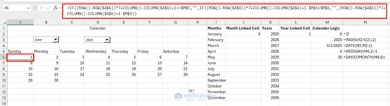
The calendar grid will use a combination of formulas to determine what date (if any) should appear in each cell.

• Select cell A6 and insert the following formula.
• Drag the formula from A6 to G11.

=IF((ROW()-ROW($A$6))*7+COLUMN()-COLUMN($A$6)+1<=$M$5,"",IF((ROW()-ROW($A$6))*7+COLUMN()-COLUMN($A$6)+1-$M$5>$M$6,"",(ROW()-ROW($A$6))*7+COLUMN()-COLUMN($A$6)+1-$M$5))

This formula generates the correct date numbers for each cell in the calendar grid:

• It calculates the day number to display in each cell based on its position in the grid.
• If the cell is before the first day of the month (<=$M$5), it stays blank.
• If the calculated day number is greater than the number of days in the month (>$M$6), it stays blank.
• Otherwise, it displays the correct day number for that date cell.

Step 5: Apply Format and Style

• Select row 5 (A5:G5) >> apply bold formatting.
• Add background color light blue.
• Select the calendar range (A6:G11).
• Apply borders:
  • Go to the Home tab >> select Borders >> select All Borders.
• Center align the text:
  • Go to the Home tab >> select Alignment >> select Center.
• Set row height to 25 for better visibility.

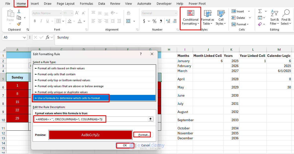
Step 6: Apply Conditional Formatting

Conditional Formatting for Weekends:

• Select the calendar range (A6:G11).
• Go to Home tab >> select Conditional Formatting >> select New Rule.
• Select Use a formula to determine which cells to format.
• Insert the following formula:

=AND(A6<>"", OR(COLUMN(A6)=1, COLUMN(A6)=7))

• Set the format to red background and white font for weekends.
• Click OK.

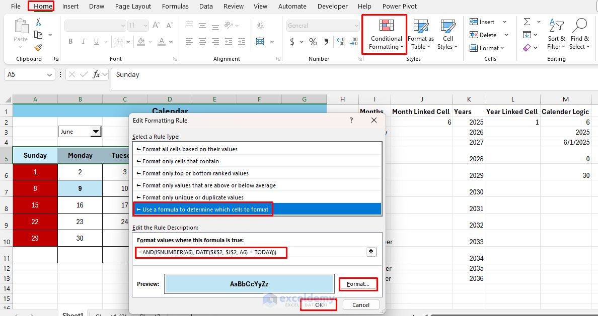
Conditional Formatting for Current Date:

• Select calendar range.
• Create another conditional formatting rule.
• Insert the following formula:

=AND(ISNUMBER(A6), DATE($K$2, $J$2, A6) = TODAY())

• Set format to bold with a light blue background.
• Click OK.

Hide Calendar Calculations:

• Select helper columns (e.g., I, J, K, L, and M).
• Right-click >> select Hide.

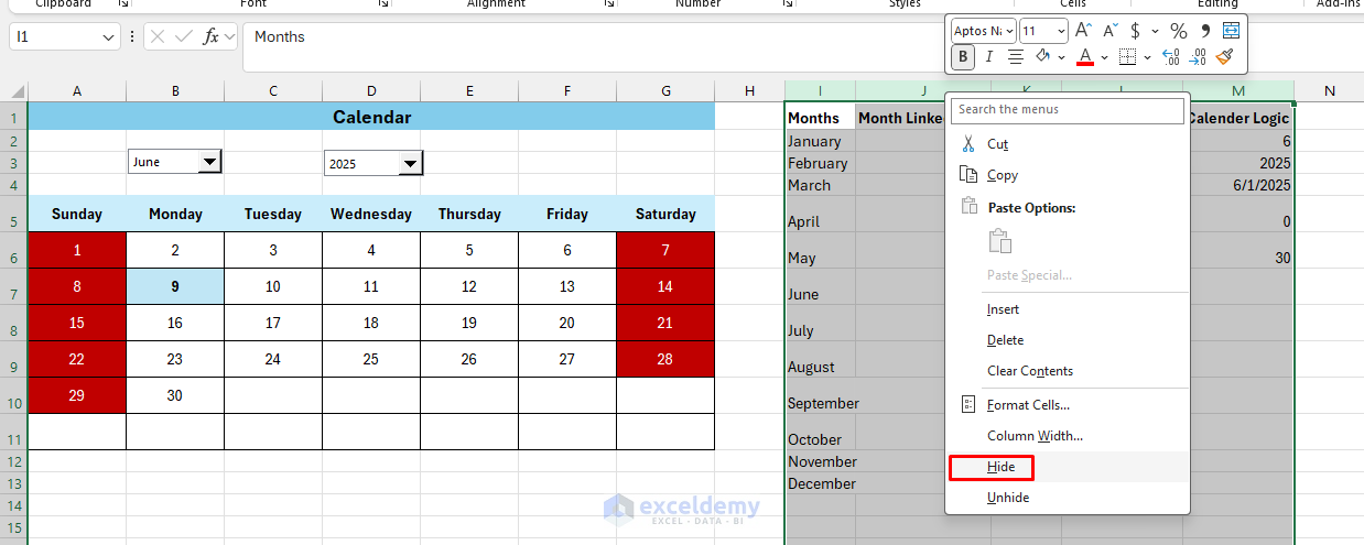
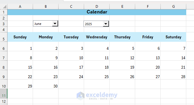
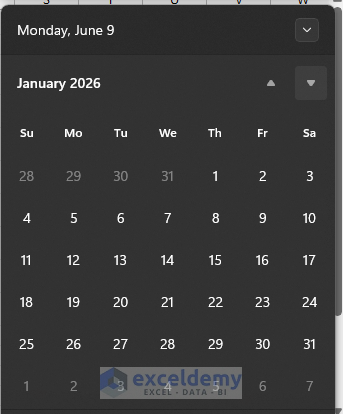
Final Calendar Interface:

Step 7: Test Calendar

• Select different months and years.
  • January
  • 2026

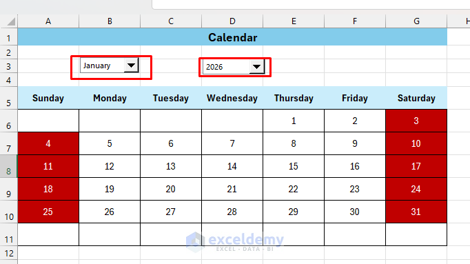
• Verify the Excel calendar with the existing calendar.

Conclusion

Following the above steps, you can build a full calendar interface in Excel using form controls. It will be a single-sheet Excel calendar where you can select the month and year from dropdowns, and the calendar automatically updates. This calendar is interactive and can be extended for years. Once you are comfortable with the basic structure, you can add features like appointment scheduling, color-coded events, or integration with other Excel data sources.